01 Automated Spectral Workflow

Installation

If you need to install AutoSpectral, run this bit first:

# Install Bioconductor packages
if (!requireNamespace("BiocManager", quietly = TRUE))
  install.packages("BiocManager")
BiocManager::install(c("flowWorkspace", "FlowSOM"))

# You'll need devtools or remotes to install from GitHub.
install.packages("remotes")
remotes::install_github("DrCytometer/AutoSpectral")

For significantly faster processing, we also recommend installing the companion C++ acceleration package. This is optional but has a meaningful effect on runtime, particularly for the automated spectral extraction and per-cell autofluorescence steps. On Windows, install Rtools first.

remotes::install_github("DrCytometer/AutoSpectralRcpp")

Once installed, AutoSpectralRcpp is used automatically wherever it helps — no further action is needed.

Get the data

Download the data for today’s example from Mendeley Data.

These data are a 7-colour panel run on a 5-laser Cytek Aurora. The samples are from spleen, lung and liver. This is a pretty simple experiment, which is nice since it will run quickly. The different tissues allow us to look at how to handle diverse autofluorescence profiles. I’ll point out that this panel has been deliberately designed to accommodate autofluorescence peaks, so we can expect autofluorescence removal to work pretty well with any method.

Start-up

Now we can load AutoSpectral.

library(AutoSpectral)

Getting your fluorophore spectra from the controls

Creating the Control File

Since the default cytometer is the Aurora, we can actually just call this without any arguments. Otherwise you need to specify the cytometer you’re using.

asp <- get.autospectral.param(
  cytometer = "aurora",
  figures = TRUE # plot figures throughout to show what's going on
)

Where are the controls? This must be typed correctly.

control.dir <- "./Raw/Set1/Reference Group"

Create the control file. You will need to manually edit your control file, telling AutoSpectral what’s going on. It will try to fill in some stuff for you, but you should check this. See the article on this on GitHub or Colibri Cytometry.

create.control.file(control.dir, asp)

We get warnings because I’ve got both bead and cell controls, and AutoSpectral would like me to pick one per fluorophore. It’s better to have only one control per fluorophore because we’ll use the spectral profiles matrix for unmixing, and if you have two instances of the same thing, that will create a big mess.

Here’s what the control file looks like as first generated:

Fill in or verify the marker, fluorophore, control.type, and universal.negative columns as appropriate. For more detail, see the Control File article.

In the automated workflow you do not need to fill in gate.name or gate.define. Those columns are only used by the legacy gating pipeline. The channel column for the peak emission channel (or one that receives a lot of signal) is also optional in the automated pipeline. The peak channel will be automatically determined from the data.

Here’s what a completed control file should look like for this workflow:

Once you’ve got it the way you want, write in the name of the control file and run the error checking function.

control.file <- "fcs_control_file.csv"
check.control.file(control.dir, control.file, asp)

This will either tell you it didn’t find any issues, or, more likely, provide you with a table of potential issues to consider fixing. Items listed as warnings will not prevent the pipeline from running, but may reduce the accuracy of the spectra generated and are things for you to check. For instance, AutoSpectral will check how many events you have in each of your control files and will raise a flag if you don’t have at least 5000 events. See the help using ?check.control.file.

Automated Spectral Extraction

The automated workflow replaces the three-step legacy pipeline (define.flow.control → clean.controls → get.fluorophore.spectra) with a single call:

spectra <- get.spectra.automated(
  control.dir     = control.dir,
  control.def.file = control.file,
  asp             = asp
)

Under the hood, get.spectra.automated() performs several in-place cleaning steps automatically, without requiring you to define or tune any gates:

1. Saturation removal — detector-saturated events are excluded before any per-fluorophore processing begins.
2. Singlet gating — doublets are automatically excluded.
3. AF orthogonalisation — for each single-stained control, the autofluorescence vector (from the paired universal.negative specified in your control file, or estimated internally from the lower quartile of the control itself) is projected out to identify events whose signal is genuinely driven by the fluorophore rather than background.
4. Cosine-similarity filtering — top-expressing candidate events are ranked by their cosine similarity to the AF vector. Events that are too AF-like are excluded, retaining only the most fluorophore-rich subset.
5. KNN scatter-matched AF subtraction — for each retained event, the nearest-neighbour unstained events in scatter space are averaged and subtracted, giving a per-event background-corrected spectral signature.
6. Automated QC with legacy pipeline fallback — the resulting spectrum is compared against the spectral reference library (via cosine similarity). If the similarity is below the default threshold, the function automatically re-runs that particular control using the original AutoSpectral pipeline with control cleaning and robust linear modelling along the expected peak channel rather than reporting a failure. If the legacy approach produces a spectrum more like the reference spectrum, that one is kept. In the event of a fallback check, both versions of the spectrum are saved for you to inspect.

The default settings work well across a wide range of panels, but the key parameters can be adjusted if needed:

spectra <- get.spectra.automated(
  control.dir           = control.dir,
  control.def.file      = control.file,
  asp                   = asp,
  n.candidates          = 1000L,   # candidate events selected per fluorophore
  n.spectral            = 200L,    # events retained after cosine filtering
  k.neighbors           = 2L,      # scatter neighbours for AF subtraction
  cosine.threshold      = 0.9,     # min cosine vs reference library
  peak.signal.threshold = 0.5      # min normalised signal in expected peak channel
)

Outputs

When figures = TRUE (the default), get.spectra.automated() produces several diagnostic outputs:

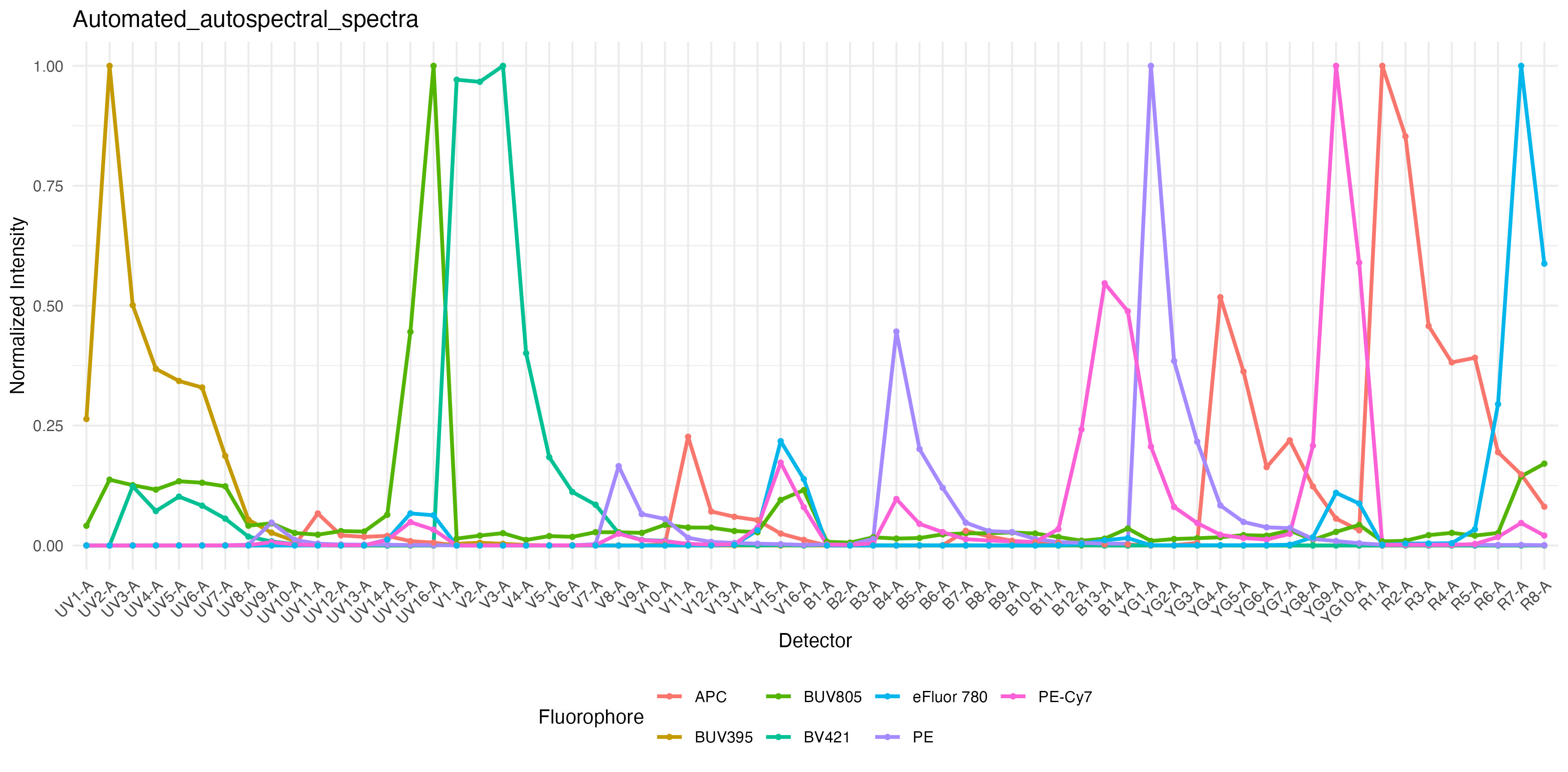
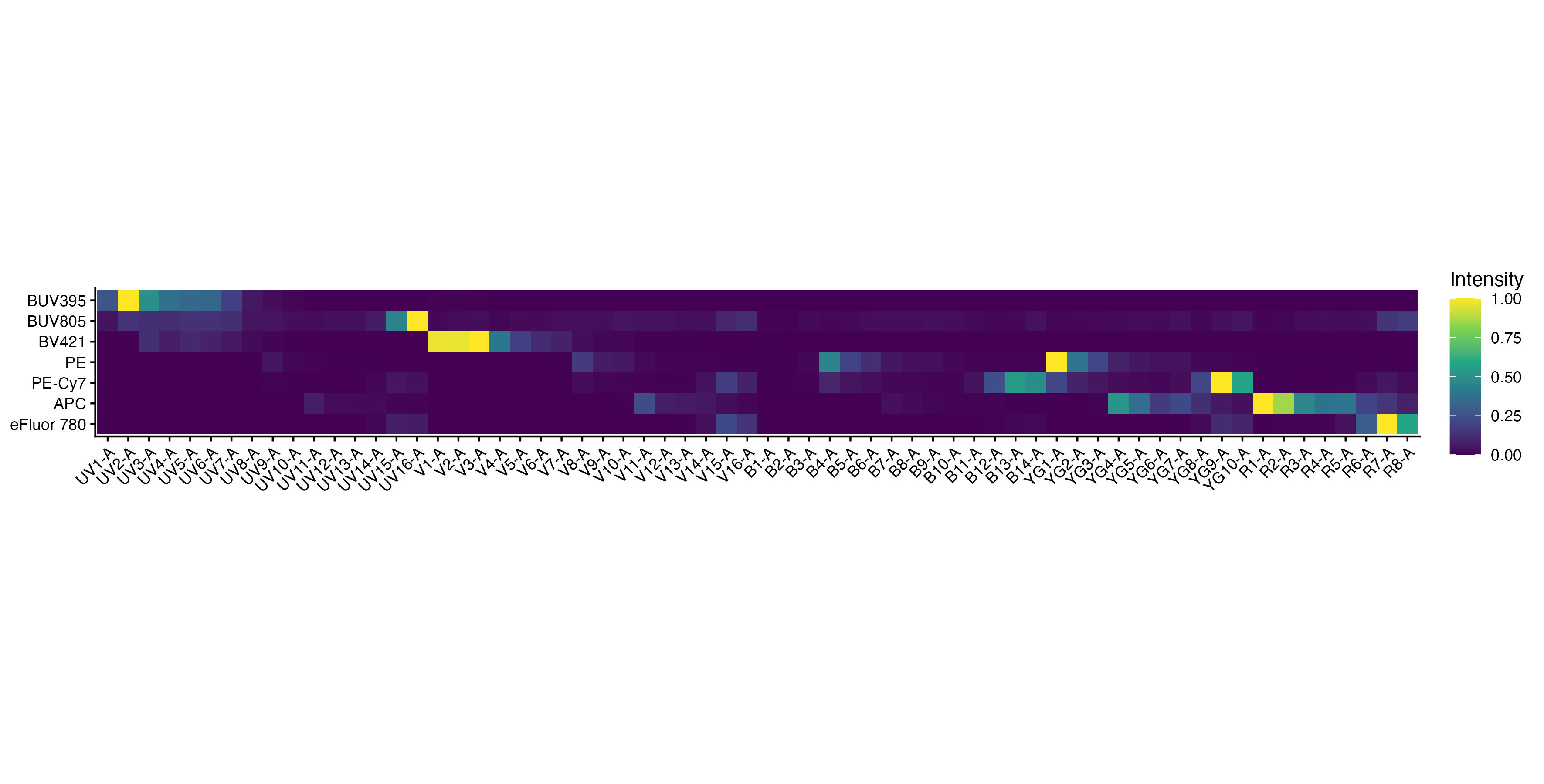
Spectral traces and heatmap (figure_spectra/) — the same standard outputs as the legacy pipeline. Check these against the expected profiles for your cytometer in online viewers such as Cytek Cloud or in the QC plots.

Spectral Signature Traces

Spectral Signature Heatmap

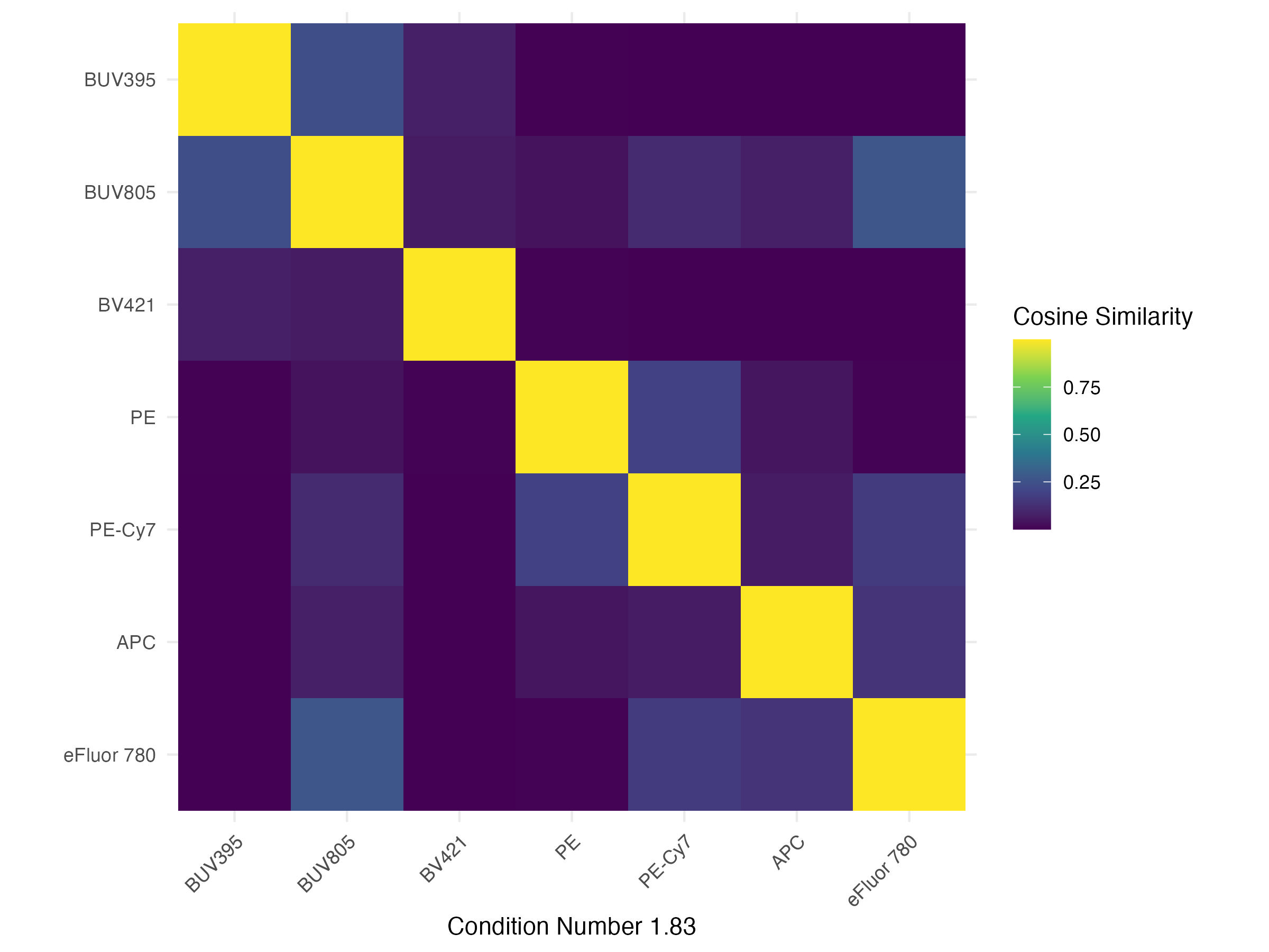
Cosine similarity heatmap (figure_similarity_heatmap/) — shows pairwise similarity between all fluorophore spectra.

Cosine Similarity Heatmap

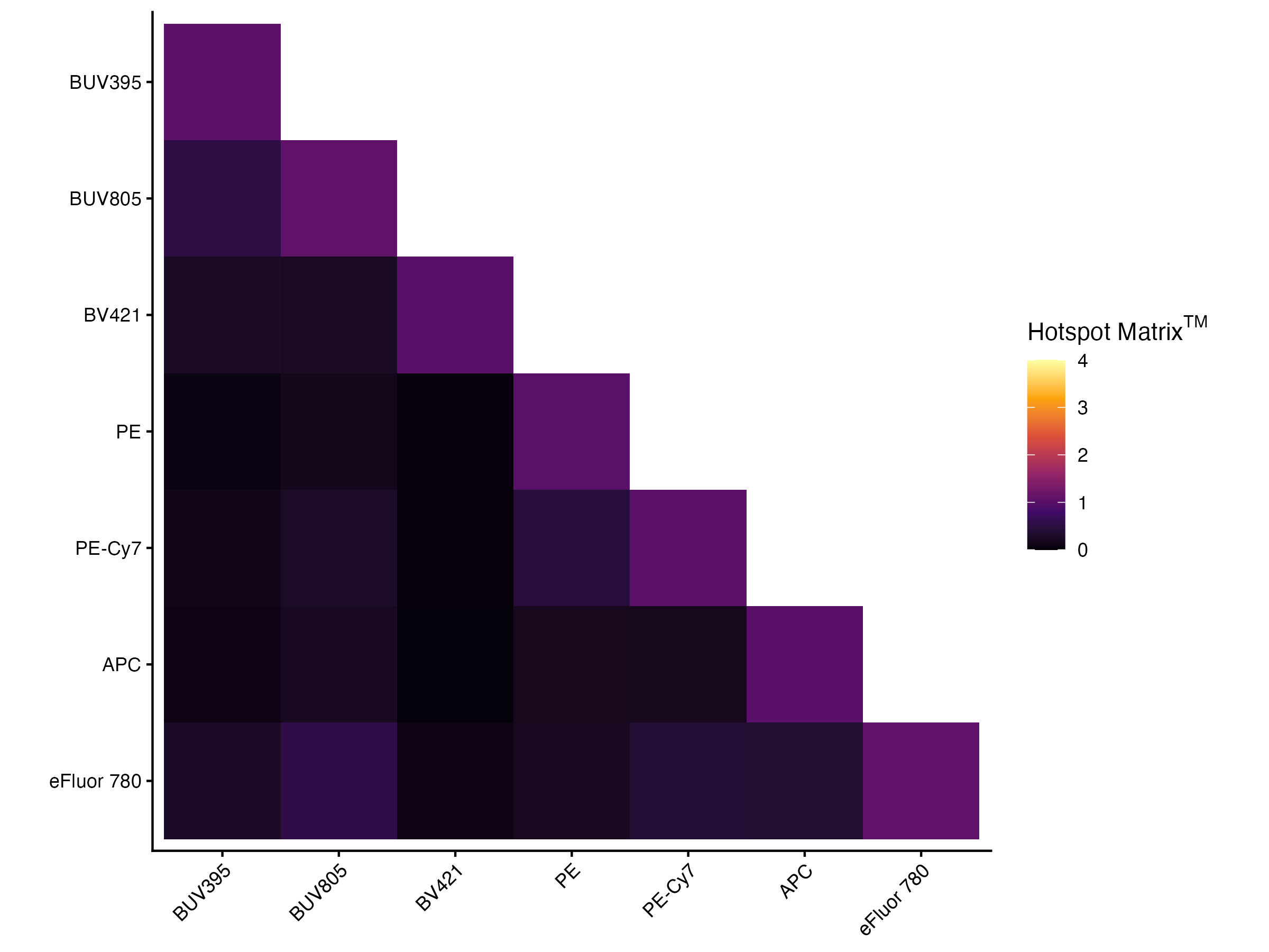
Hotspot matrix (figure_similarity_heatmap/) — highlights fluorophore pairs with high spectral overlap, as in Mage et al. Values above 6 are most likely to cause unmixing problems; values between 4 and 6 are worth reviewing.

Hotspot Matrix Heatmap

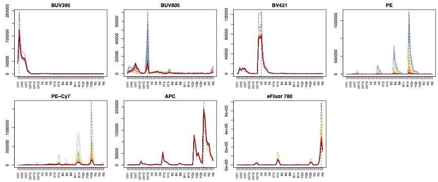
Per-fluorophore cosine-filter traces (figure_spectra/) — a multi-panel PDF showing, for each control, how events are distributed by their cosine similarity to the AF vector. Quantiles are coloured from least (blue) to most (red) AF-like. This is a very quick, automated approach to intrusive AF noise exclusion that takes the place of the gating-based exclusion in AutoSpectral <1.6.0. You’ll notice that the brightest events are typically the cleanest, as should be expected (they are farthest from background).

Hotspot Matrix Heatmap

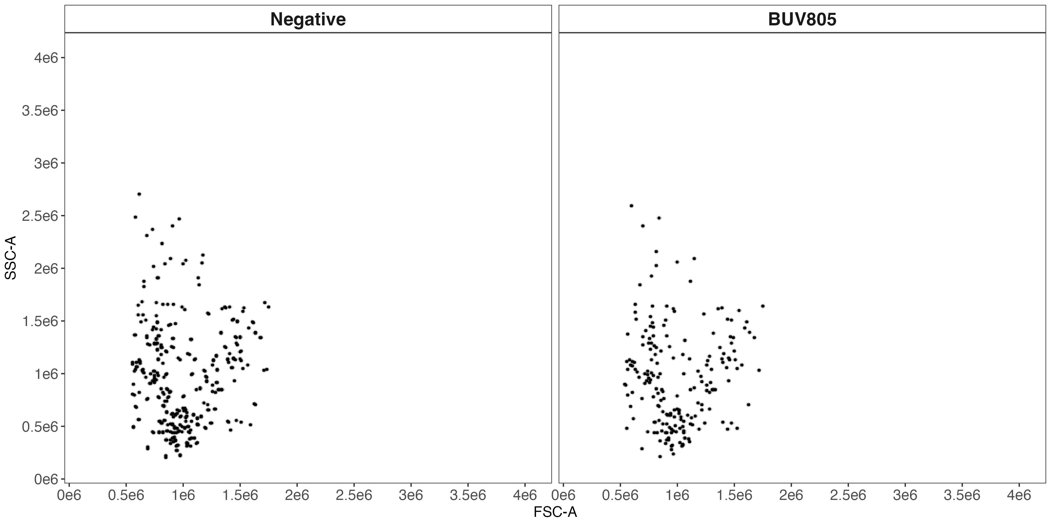
Scatter-match plots (figure_scatter_match/) — a multi-panel PDF showing, for each fluorophore, the unstained background population, the selected spectral events, and the matched AF/negative events used for subtraction. This is now done using k-nearest neighbours, and should be essentially perfect. Here’s CD11b - BUV805:

Hotspot Matrix Heatmap

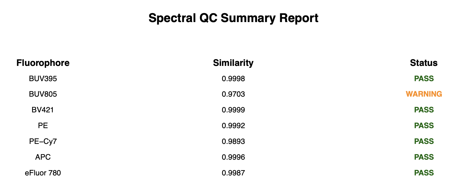
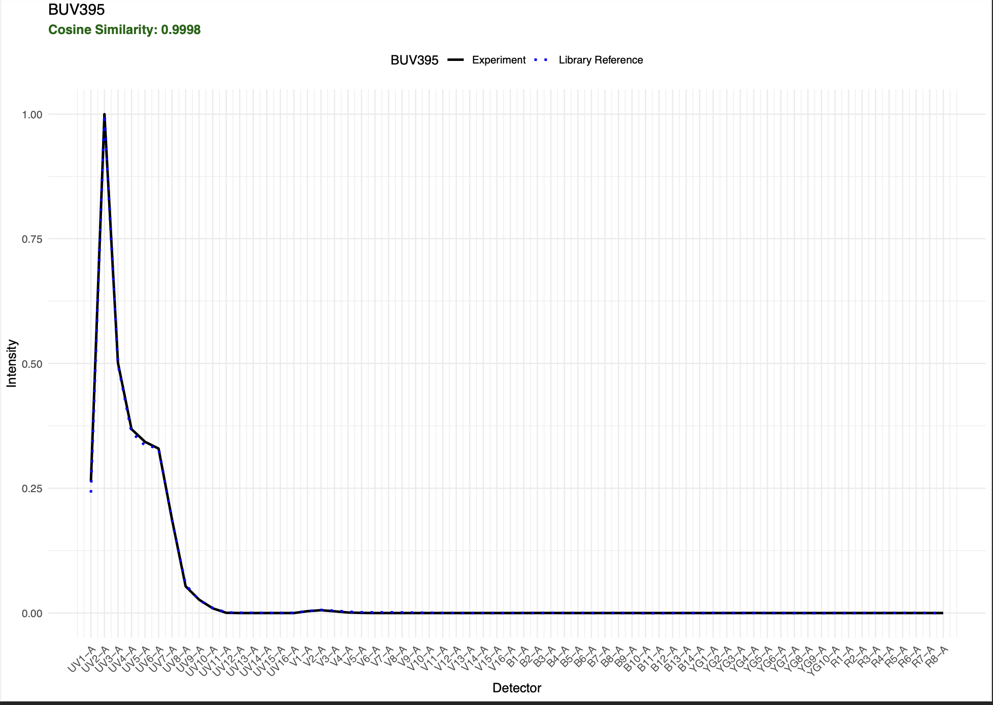
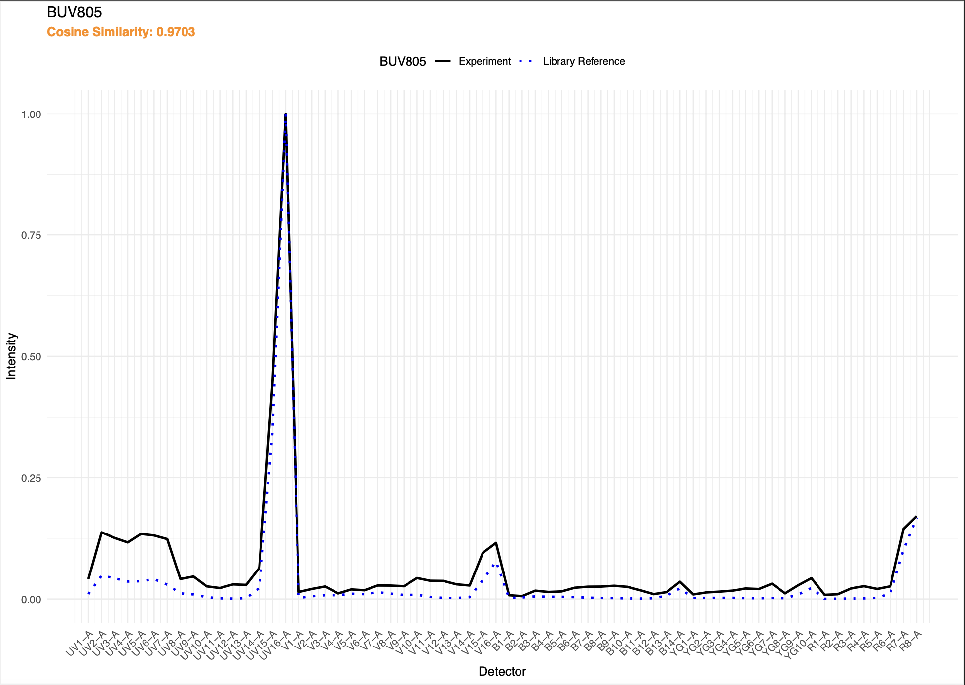
Spectral QC report (figure_spectral_ribbon/) — a per-fluorophore PDF comparing the extracted spectrum against the reference library entry for that instrument. Fluorophores that triggered the RLM fallback are flagged, and both the automated and refined spectra are shown where applicable.

Spectral QC Report

Spectral QC BUV395

Spectral QC BUV395

Spectra CSV — the final normalised spectra matrix is saved to table_spectra/. You can reload it later using read.spectra() and pass it directly to any unmixing function. Call list.files("table_spectra/") to find all the files in that folder.

By default, the new spectral profile extraction pipeline does not include any autofluorescence parameter in the output spectra. This is to try to reduce confusion. If you want a single AF, as you might have in SpectroFlo or other software, you can set return.af=TRUE in the call to get.spectra.automated(). This will extract the mean AF background in the unstained sample that you label as “AF” in the fluorophore column of your control file.

Note for ID7000 users: because the ID7000 can be set up with basically any voltage settings for the controls, the spectral signatures are really not very consistent between machines (in my experience). So, the spectral references in AutoSpectral will not be very informative. In order to avoid having all of the “mismatches” trigger legacy refinement, the thresholds for this are relaxed for ID7000 files. This should be fine, since the new automated pipeline tends to be at least as accurate as the legacy approach.

Details: get.spectra.automated() Parameter Reference

Parameter	Default	What it does
control.dir	—	Path to the directory of single-stained control FCS files.
control.def.file	—	Path/filename of the control definition CSV. Must already pass check.control.file().
asp	—	The AutoSpectral parameter list from get.autospectral.param().
n.candidates	1000L	Top-expressing candidate events selected per fluorophore before cosine filtering. Ignored in internal-negative mode (no paired universal.negative file), where the top 5% of events by peak channel are used instead.
n.spectral	200L	Number of spectral events retained after cosine-similarity filtering against the AF vector.
k.neighbors	2L	Number of nearest neighbours in scatter space used for per-event AF subtraction (KNN scatter-matched AF subtraction step).
singlet.quantiles	c(0.85, 0.975)	Quantile range used for doublet discrimination on the FSC-H/FSC-A (and SSC) ratio. Tighten this range if you suspect doublet contamination is still getting through.
cosine.threshold	0.9	Minimum cosine similarity against the spectral reference library required to accept the automated spectrum. Anything below this triggers legacy-pipeline refinement (see note above for ID7000 data).
peak.signal.threshold	0.5	Minimum normalised signal expected in the peak detector. Informational QC only — it’s reported in the QC log but does not itself trigger legacy refinement.
legacy.refinement	TRUE	Whether to fall back to the legacy define.flow.control → clean.controls → get.fluorophore.spectra pipeline for any fluorophore that fails the cosine QC check. Set to FALSE if you’d rather just see the QC failures and handle them manually.
top.expressing.override	NULL	A named numeric vector to override the candidate-event count for specific controls (e.g. c("BUV805" = 500)). Names can be the FCS filename (no extension) or the fluorophore name. Useful for a control with unusually low event counts or very few positives.
return.af	FALSE	Appends a single mean-AF row (named "AF") to the output spectra matrix, for use with plain OLS/WLS unmixing. Requires a control row with fluorophore = AF.
figures	TRUE	Produces the full set of diagnostic plots (spectral trace, heatmap, cosine-similarity heatmap, hotspot matrix, QC report).
plot.cosine.filter	TRUE	When figures = TRUE, also generates the multi-panel cosine-similarity filter PDF (per-fluorophore, binned by AF-likeness). Turn off to save time on large panels.
plot.scatter.match	TRUE	When figures = TRUE, also generates the multi-panel KNN scatter-match PDF. Turn off to save time on large panels.
verbose	TRUE	Print progress messages and the final QC summary table to the console.

Tips:

• If you’re getting a lot of LEGACY_REFINEMENT flags, check peak.signal.threshold and cosine.threshold together in the QC log before assuming your controls are bad. A genuinely dim control will show low PeakSignal as well as low CosineSim.
• n.candidates and n.spectral only matter in external-negative mode (i.e. where a universal.negative file is paired with the control). In internal-negative mode, the top-5%/bottom-10% event split is fixed and these two parameters are silently ignored.
• The function always writes two CSVs to table_spectra/: Automated_<name>.csv (best-choice, may include legacy-adopted spectra) and Automated_original_<name>.csv (always all-automated). If you’re benchmarking the automated pipeline itself, use the _original_ file so legacy fallbacks don’t skew your comparison.

Unmixing

AutoSpectral provides options for unmixing. Let’s start with the most basic, which is replicating the OLS unmixing as in SpectroFlo (this is Aurora data). By default, the automated spectral extraction pipeline does not provide an autofluorescence signature, so this will be comparable to performing unmixing without autofluorescence extraction. Autofluorescence is best handled via the per-cell approach detailed below.

We need a minimal flow.control object for feeding in the dye and marker names during unmixing. In the automated workflow, this is created using the reload.flow.control() tool:

flow.control <- reload.flow.control(
  control.dir      = control.dir,
  control.def.file = control.file,
  asp              = asp
)

To unmix, specify the file (and path) of the FCS file you want to unmix:

spleen.fcs.file <- "./Raw/Set1/Stained/D4 Spleen_Set1.fcs"
unmix.fcs(
  spleen.fcs.file,
  spectra,
  asp,
  flow.control,
  method = "OLS",
  file.suffix = "without AF extraction"
)

Note that this is just using OLS–this is not the “AutoSpectral” unmixing method, we are just using the AutoSpectral R package to perform bog standard unmixing.

If we have a folder full of FCS files, we can do all the files in the folder. Note that this is essentially just an lapply loop over the files. It can, however, be parallelized (set parallel=TRUE). Memory usage is handled via file chunking, which you can modify using the chunk.size argument, if needed.

unmix.folder(
  fcs.dir = "./Raw/Set1/Stained/",
  spectra = spectra,
  asp = asp,
  flow.control = flow.control,
  method = "OLS" # use OLS unmixing (not AutoSpectral unmixing)
)

By default, the unmixed files are generated in Autospectral_unmixed, but you can change that by passing a path to output.dir.

If we want to use weighted least-squares, we call like this:

unmix.fcs(spleen.fcs.file, spectra, asp, flow.control, method = "WLS")

More details on WLS unmixing, including calculating and re-using weights are detailed in dedicated article

Okay, that’s basic unmixing. And, I think you should see a bit of improvement using AutoSpectral even with the same unmixing algorithms due to the improvements in single-colour control handling. We do.

Per-cell unmixing

Per-cell Autofluorescence Extraction

For per-cell autofluorescence extraction and per-cell fluorophore optimization, AutoSpectral needs more information. We will extract autofluorescence signatures from the three tissues involved here, and look at how to use those in the unmixing. We’ll also get information about the fluorophore emission variability and use that to try to improve the unmixing.

When we go to use this information in the unmixing, we select method = AutoSpectral.

Per-cell autofluorescence extraction is substantially faster with AutoSpectralRcpp installed (see the Installation section above). Once installed, it takes over automatically — no further action is needed.

To use per-cell autofluorescence extraction only, no fluorophore optimization, do this:

spleen.unstained <- "./Raw/Set1/Unstained/D1 Spleen_Set1.fcs"
spleen.af <- get.af.spectra(
  unstained.sample = spleen.unstained,
  asp = asp,
  spectra = spectra,
  refine = TRUE # optional; when TRUE, more AF spectra will be generated, focusing on problem cells. This takes longer, though.
)
unmix.fcs(
  fcs.file = spleen.fcs.file,
  spectra = spectra,
  asp = asp,
  flow.control = flow.control,
  method = "AutoSpectral", # use AutoSpectral unmixing
  af.spectra = spleen.af, # use these AF signatures as the options
  file.suffix = "per-cell AF extraction"
)

Using refine=TRUE will take longer, both during the get.af.spectra() call and during subsequent unmixing calls. The benefit of this is primarily in messier samples, particularly those from tissues. If you are just using PBMCs or nice lymphoid samples like spleen, you probably won’t see much benefit from this.

We get the distribution of autofluorescence spectra as a spectral trace and as a heatmap in figure_autofluorescence. The AF spectra are saved as a CSV file in table_spectra.

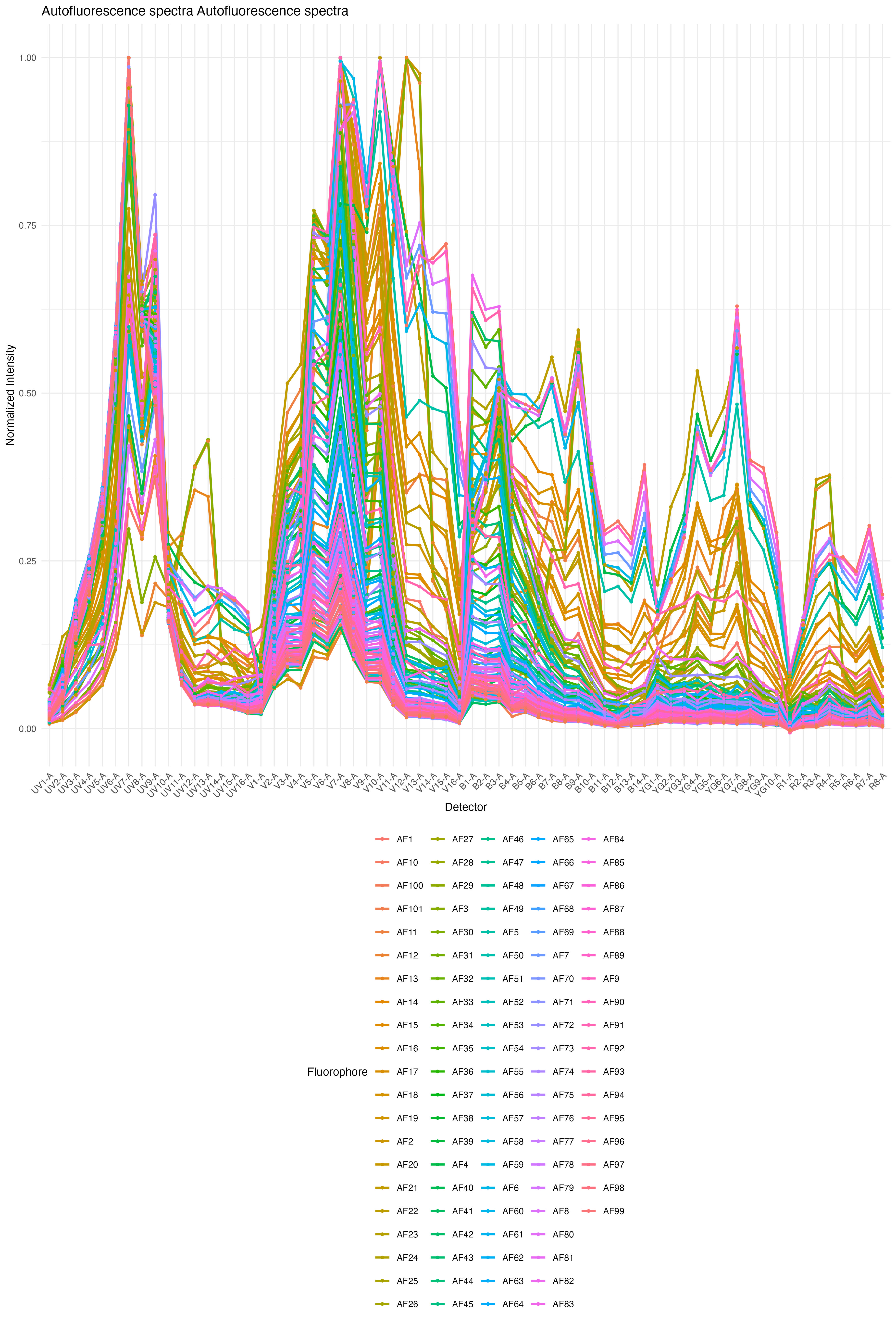
Autofluorescence profiles in the spleen

We can also look at the distribution of autofluorescence like this, where the black line represents a median signature (what you might use with an automated single AF parameter), and the red traces represents the variation:

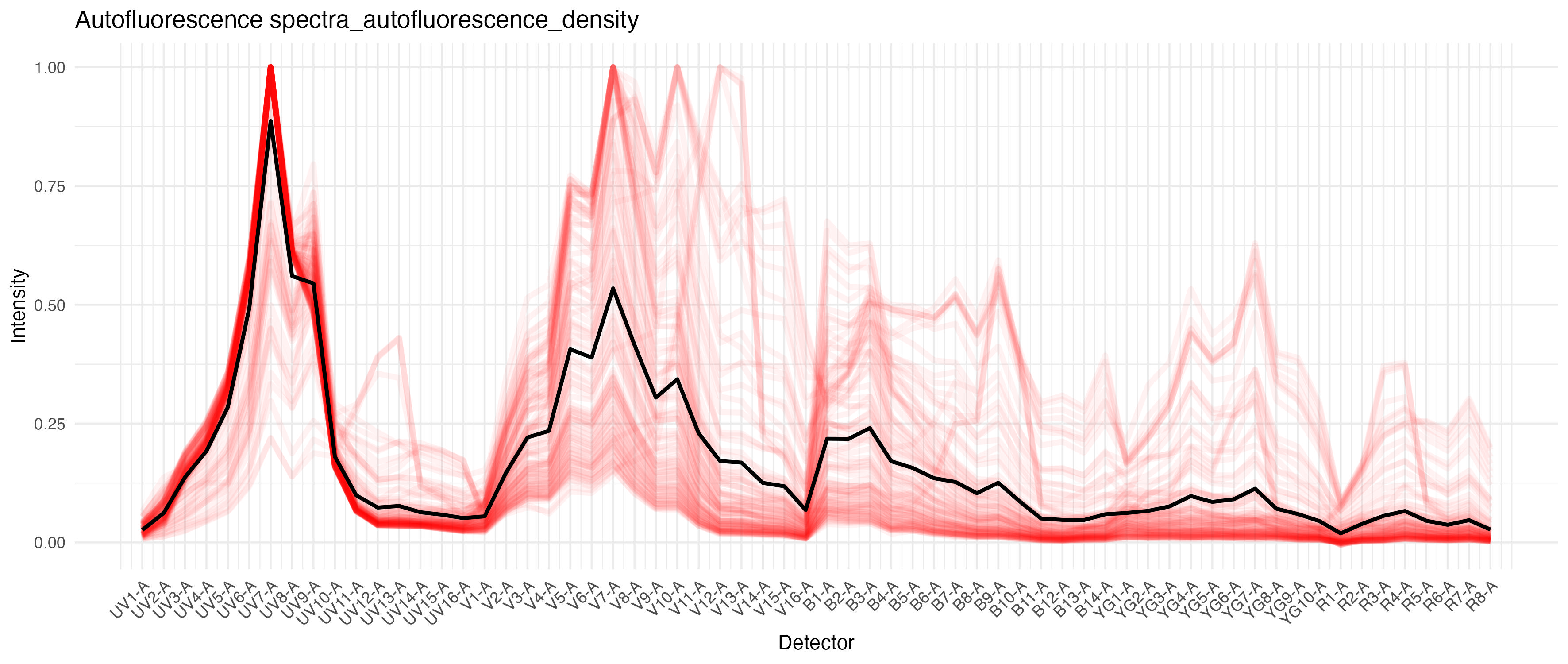
Autofluorescence variation in the spleen

We also get images showing us the impact of the AF extraction on the unstained sample we have supplied.

This is without any AF extraction, looking at what AutoSpectral has determined are the two most-affected fluorophore channels:

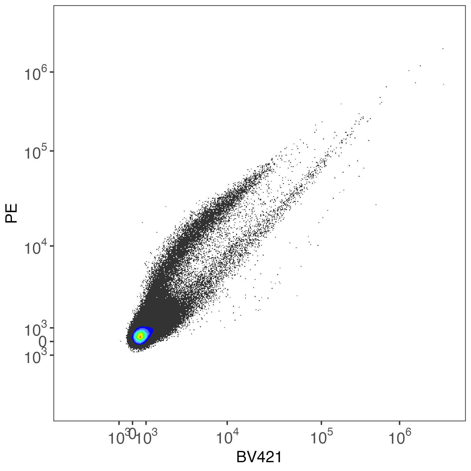
Spleen: No AF Extraction

What you get on the same unstained sample with per-cell AF extraction, without refinement (refine=FALSE):

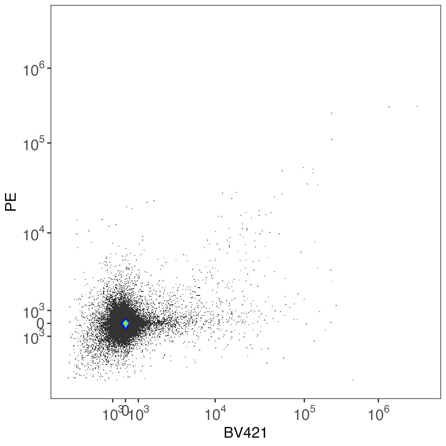
Spleen: Per-Cell AF Extraction

What you get on the same unstained sample with per-cell AF extraction, with refinement (refine=TRUE):

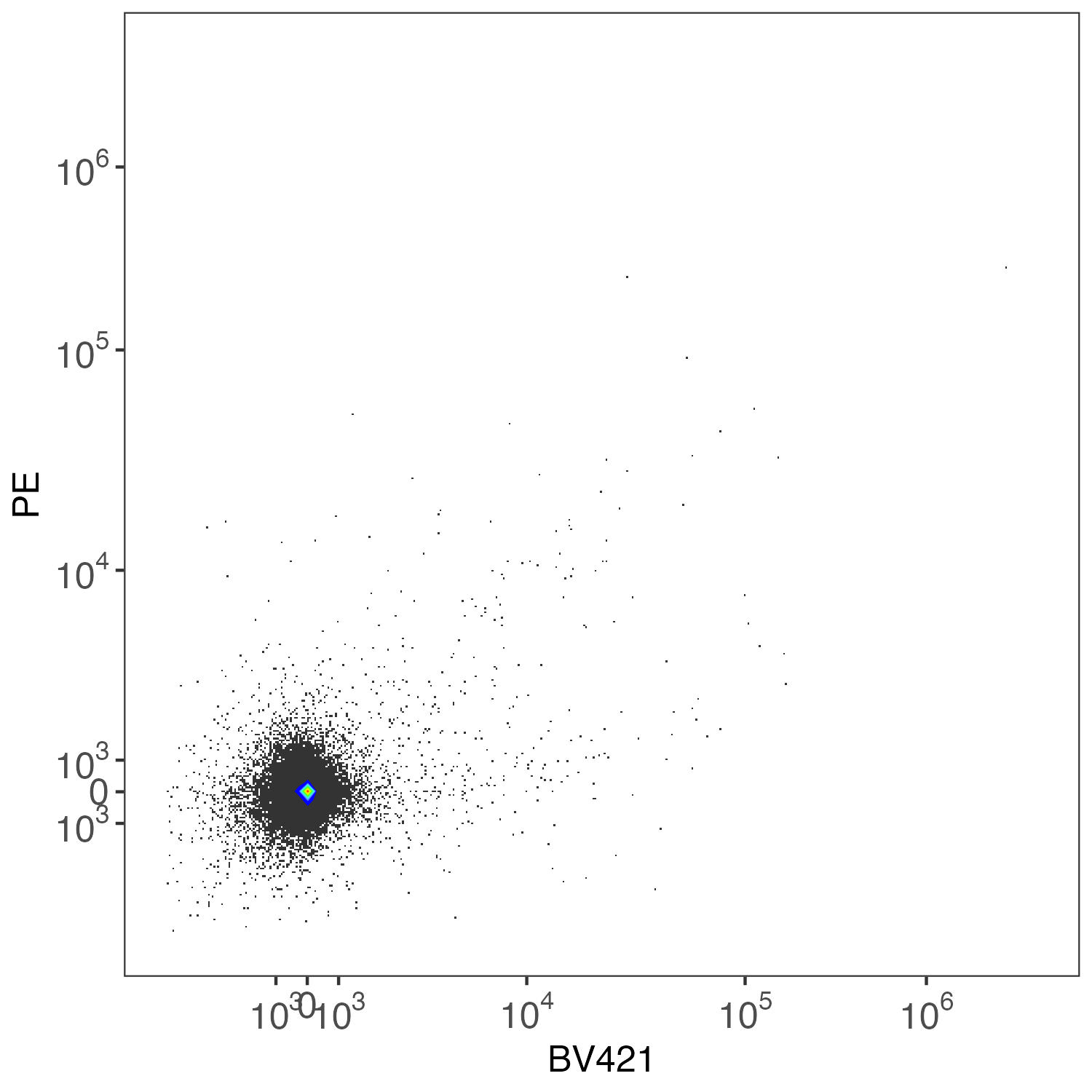
Spleen: Per-Cell AF Extraction Refined

If you want to do this with samples containing different autofluorescence profiles, such as we have here, we extract the AF spectral variation from each type of unstained sample. We then provide the corresponding af.spectra to each unmixing call. The unmixing call can be to a single FCS file, or it can be, as above, to a folder. So, if you have a whole set of stained lung samples, you’d pull your AF spectra from the unstained lung sample, and then call unmix.folder on the folder containing your lung (and only lung) samples. Repeat for each type of autofluorescence sample. Read more about how the per-cell autofluorescence extraction works in the GitHub or Colibri article.

In this case, we have three types of samples: spleen, liver and lung tissues. If you are working with human PBMCs, usually a single (optionally pooled) unstained PBMC sample is fine. If, however, you have samples from very sick donors, you might consider collecting unstained sample from each donor and matching the autofluorescence more closely. This is easier to set up in the Honeychrome app, where you can quickly assign and inspect the results in a visual interface.

lung.unstained <- "./Raw/Set1/Unstained/D2 Lung_Set1.fcs"
lung.af <- get.af.spectra(lung.unstained, asp, spectra) # use refine=TRUE for a modest improvement, default is FALSE
lung.fcs.file <- "./Raw/Set1/Stained/D5 Lung_Set1.fcs"
unmix.fcs(
  lung.fcs.file,
  spectra,
  asp,
  flow.control,
  method = "AutoSpectral",
  af.spectra = lung.af,
  file.suffix = "per-cell AF extraction"
)

liver.unstained <- "./Raw/Set1/Unstained/D3 Liver_Set1.fcs"
liver.af <- get.af.spectra(liver.unstained, asp, spectra) # use refine=TRUE for a modest improvement, default is FALSE
liver.fcs.file <- "./Raw/Set1/Stained/D6 Liver_Set1.fcs"
unmix.fcs(
  liver.fcs.file,
  spectra,
  asp,
  flow.control,
  method = "AutoSpectral",
  af.spectra = liver.af,
  file.suffix = "per-cell AF extraction"
)

You can easily set this up as a for loop or an lapply loop matching elements by names from a list.

For more detail on the per-cell AF extraction, see the dedicated article on this subject.

Per-cell Fluorophore Optimization

To do per-cell fluorophore optimization, we will first measure the variation in the spectrum for each fluorophore. For the unmixing, we’ll supply the af.spectra and the spectra.variants, calling AutoSpectral unmixing. Read more about how the per-cell fluorophore optimization works in the GitHub or Colibri article.

As of version 1.6.0, we no longer provide autofluorescence information via af.spectra when calling get.spectral.variants(). This is handled automatically by the function internals to avoid creating any confusion and to make it easier for you, the user.

variants <- get.spectral.variants(
  control.dir = control.dir,
  control.def.file = control.file,
  asp = asp,
  spectra = spectra,
  parallel = FALSE # use parallel if TRUE
)

The output of this is saved as an RDS file in folder figure_spectral_variants. You can load it back in using the readRDS() function in base R.

There are plots of the spectral variation for each fluorophore. For something like the CD11b-BUV805 in this data, we have some changes in the autofluorescence because there are multiple cell types expressing CD11b, but we have at least as much variation in the long wavelength spillover on the violet and red laser, as should be expected from a tandem dye.

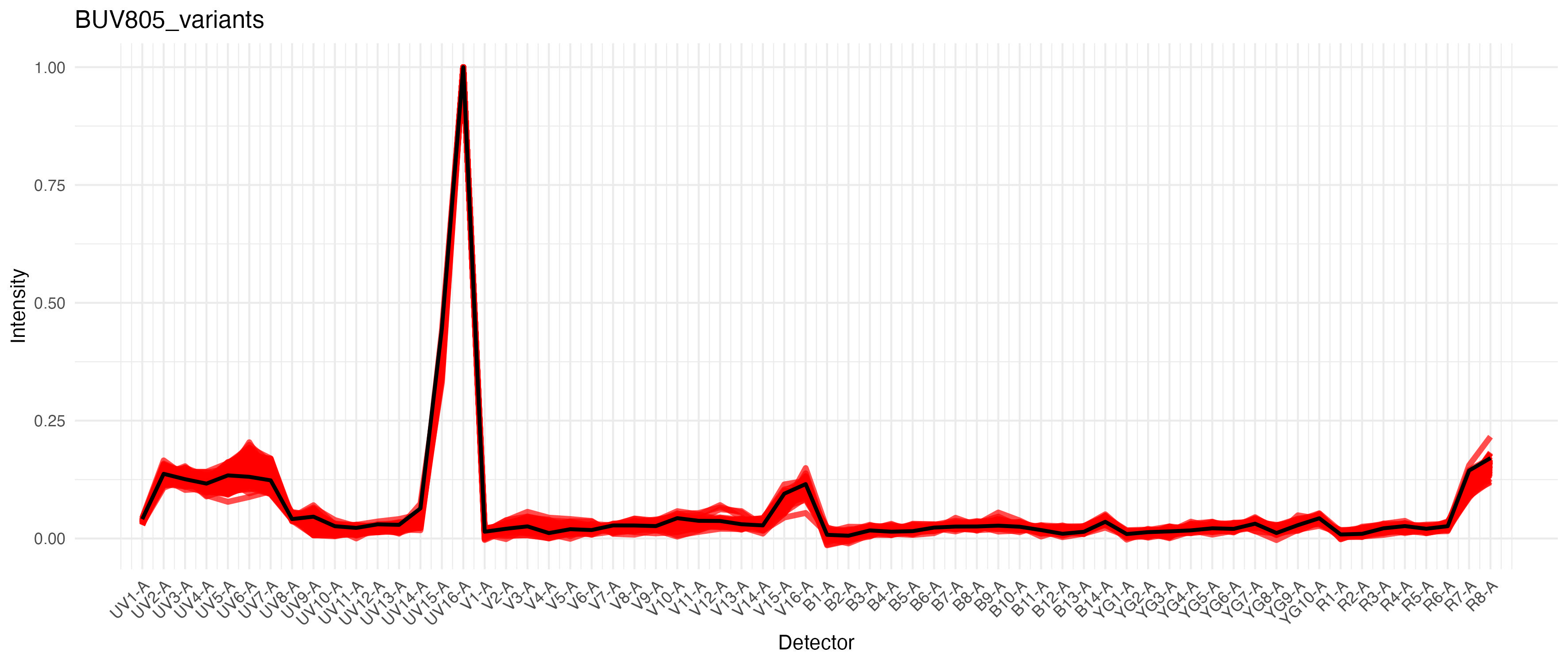
Variation in BUV805

For PE-Cy7, we get a modest difference in the excitation between the blue and yellow-green lasers, which would cause spread if we had a fluorophore in that range on the blue laser, such as RB780. We don’t in this case.

Variability in the YG1-A detector is likely tandem breakdown (variable free PE signal).

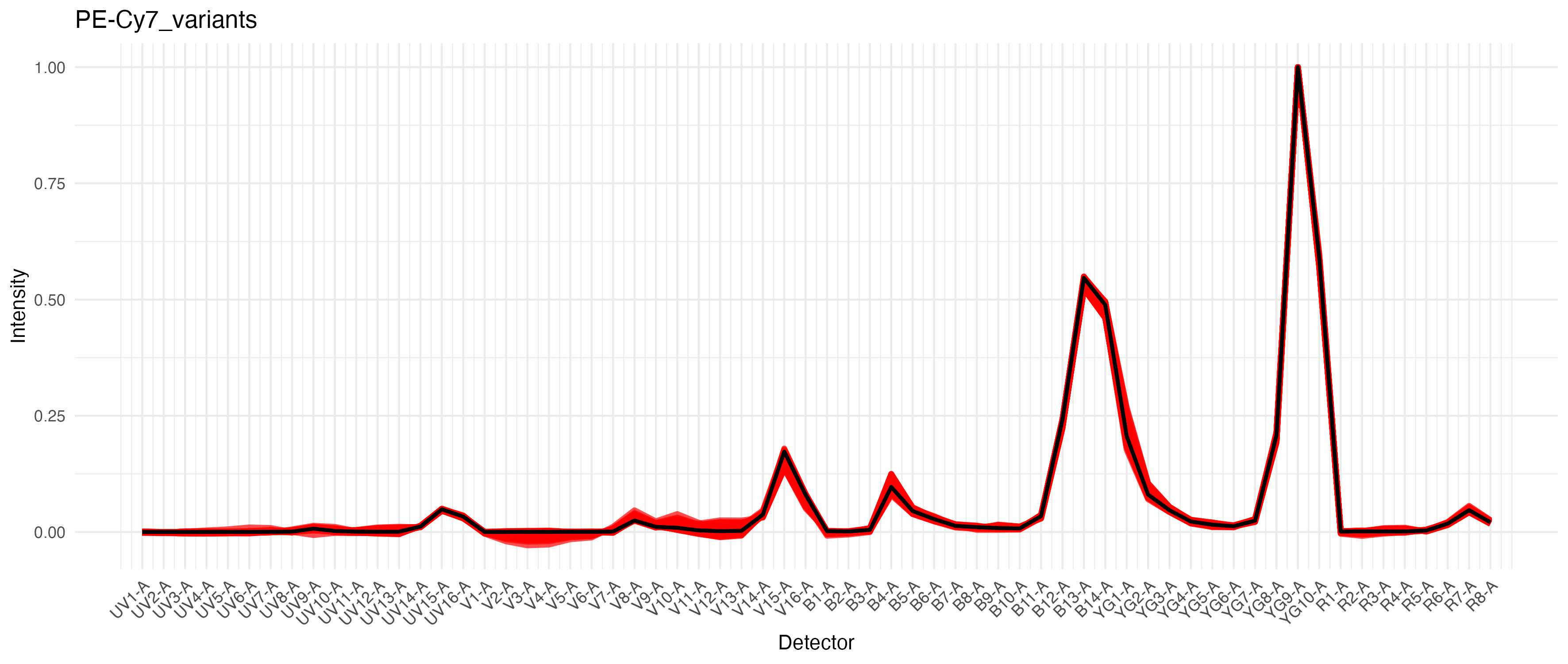
Variation in PE-Cy7

We can now pass this to the unmixing call. For quicker results, you may set the speed to fast, which checks fewer pre-screened variants per cell.

unmix.fcs(
  lung.fcs.file,
  spectra,
  asp,
  flow.control,
  method = "AutoSpectral", # use AutoSpectral unmixing
  af.spectra = lung.af, # use this set of AF (matched to sample source)
  spectra.variants = variants, # by providing variants, we instruct the unmixing to perform per-cell fluorophore optimization
  file.suffix = "per-cell AF and fluorophore optimization",
  speed = "slow", # slow will be a bit better
  parallel = TRUE
)

Please note that if you are comparing the output FCS files from AutoSpectral to others you may have from the cytometer and you are doing this in FlowJo, FlowJo V10 is still terrible at handling scales. You must set the transformations on the axes to be the same for all coefficients in order to do a fair comparison. Otherwise you’ll see whatever you’ve already done to tune your display (e.g., biexponential width basis) for your existing files versus some random default selection by FlowJo for AutoSpectral’s files. Nothing to do with me.

For more detail on the per-cell fluorophore optimization, see the dedicated article on this subject.

Plotting

You can do a comparison using the plotting functions in AutoSpectral, but a dedicated flow cytometry analysis program with a graphical interface will be better. More on plotting on the dedicated article on GitHub or Colibri.

autospectral.unmixed.lung <- "AutoSpectral_unmixed/D5 Lung_Set1 AutoSpectral per-cell AF and fluorophore optimization.fcs"
spectroflo.unmixed.lung <- "./Unmixed/Set1/Stained/D5 Lung_Set1.fcs"

# using native AutoSpectral reader here (see `flowstate`)
asp.lung <- AutoSpectral::readFCS(autospectral.unmixed.lung)
sf.lung <- AutoSpectral::readFCS(spectroflo.unmixed.lung)

create.biplot(sf.lung, "BUV395-A", "BV421-A", asp, title = "SpectroFlo")
create.biplot(asp.lung, "BUV395-A", "BV421-A", asp, title = "AutoSpectral")

Let’s have a look at the unmixed data.

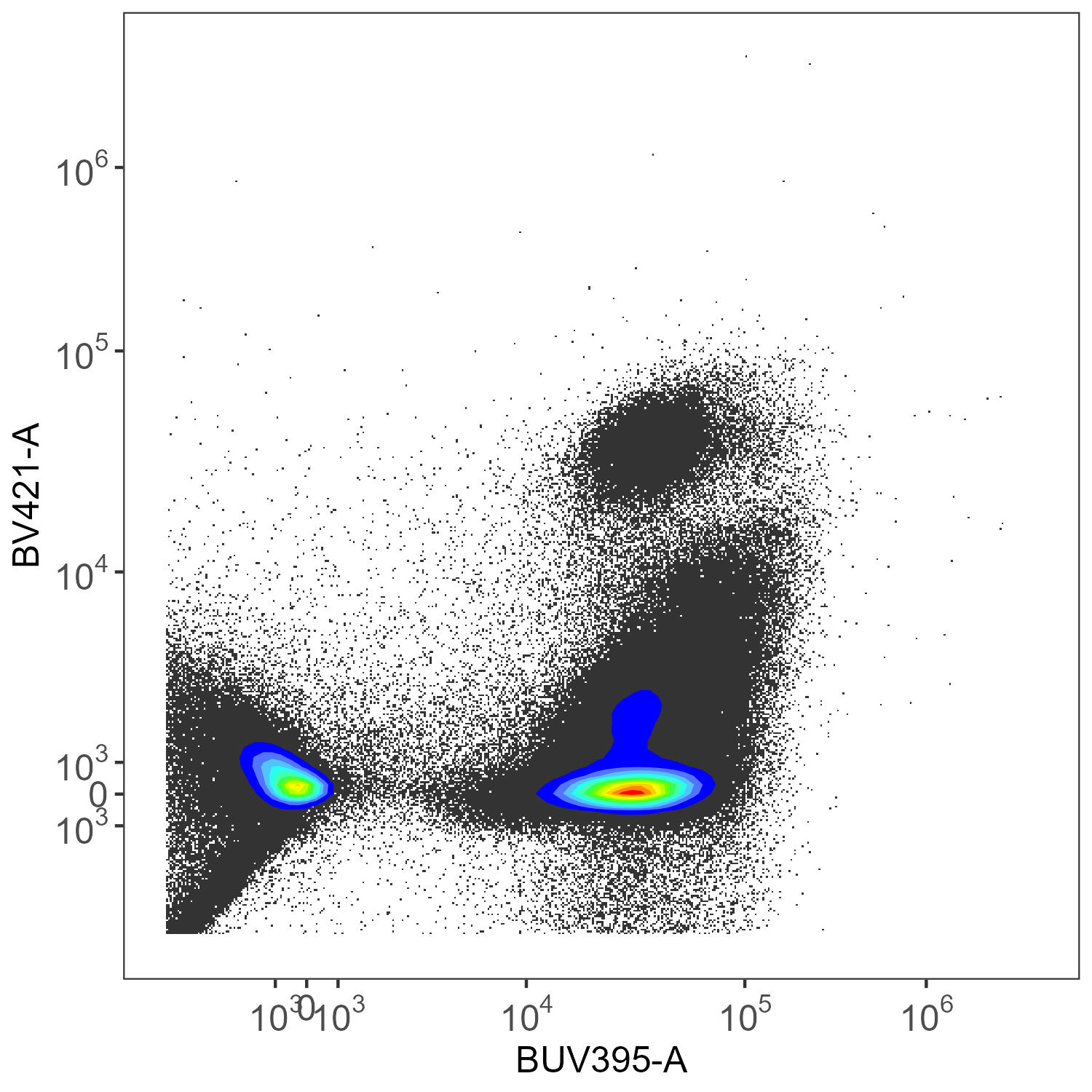
SpectroFlo Unmixed

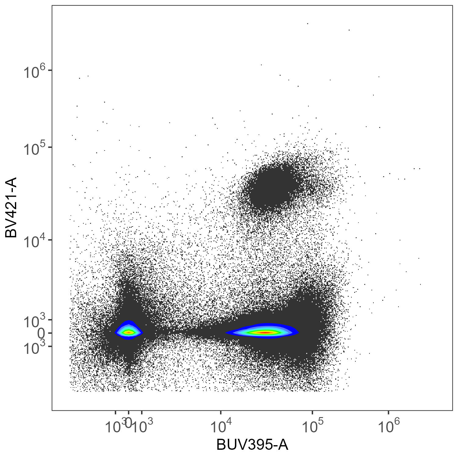
AutoSpectral Unmixed

Here we have CD45-BUV395 and CD4-BV421. There really shouldn’t be much of anything low for CD4 in the mouse. This is ungated data, so we’re seeing everything, without any clean-up.

The original unmixing only uses a single autofluorescence parameter. As mentioned at the beginning of this post, you can use multiple autofluorescence to achieve better results in SpectroFlo with this small panel as it has been designed to accommodate that. There is no one solution for that approach, though.

Also, the plots shown here have hard cut-offs on the x and y axes, determined by arguments to create.biplot(). That can be modified, of course, but as stated, you’re better off doing that in dedicated flow analysis software.