11 Per Cell Optimization

The aim of this article is to explain a bit more about how we go about optimizing the fluorophore signatures used for unmixing on a per-cell basis in AutoSpectral. Let me know if the explanation doesn’t make sense. There are days when I think it’s really weird that we can actually figure this stuff out from the data. Also, this is not the only way of doing this, just the best one I’ve found so far.

Okay, so we’re basically going to play some Tetris with your unmixing. You can also think of this as “theme and variations” if you’re musically inclined, or multiverse unmixing, if you prefer comics.

The aim here is to deal with the inherent variability that exists in the emissions from the fluorophores. This variability manifests at the level of the cell (or particle/data point) as spread. Spread is a population-level thing; individual cells do not have spread, they have exact positions. We get spread in the unmixing (and compensation in conventional flow) because we have a distribution of outcomes in the spillover/spectra for the fluorophores and we unmix using only a single (hopefully) best fit spectrum. This means there are data on both sides of that single best fit (think of it as a median or average for the distribution), both in the raw data and the unmixed. If there is a mismatch between the single-colour control used to generate the fluorophore’s spectrum and the actual data in the fully stained sample, this will manifest as a skew in the distribution of the unmixed data (i.e., unmixing error). These mismatches can occur for a multitude of reasons, including tandem breakdown, improperly prepared controls, bead-based controls, low brightness or autofluorescence (AF) contamination of the spectrum. The first part of AutoSpectral–getting the optimized single spectra using clean.controls() and get.fluorophore.spectra(), gets you as far as it can with a single spectrum per fluorophore. This is the next step.

What we are going to do is similar to what we did with the single cell AF extraction. We will start by mapping the variation in the single-color controls for each fluorophore using a self-organizing map (SOM).

library( AutoSpectral )
#> AutoSpectralRcpp detected: using Rcpp-accelerated readFCS and writeFCS.

If you haven’t already done so, you’ll need to run the basic AutoSpectral workflow to get clean spectral signatures and autofluorescence signatures. See the articles on this, including “Single Cell Autofluorescence”.

The af.spectra here should match the source of your cells in the single-colour controls. If you’re using beads for your single colour controls, the af.spectra should match the unstained sample that is provided as AF in the control.file.

For this example, we’ll assume you’ve already run AutoSpectral to extract both your fluorophore signatures and your autofluorescence spectra. This should be quick. For read.spectra(), change the name of your files as appropriate. If they aren’t in the table_spectra folder, change the location using the spectra.dir argument.

asp <- get.autospectral.param( cytometer = "aurora", figures = TRUE )
control.dir <- "./SSC"
control.file <- "fcs_control_file.csv"
spectra <- read.spectra( "Cells AF Removed autospectral spectra.csv" )
af.spectra <- read.spectra( "autospectral autofluorescence.csv" )

Now we are ready to go variant hunting.

For the variants, we’re going to load in the FCS file for each single-colour control, identify the brightest non-autofluorescent events in the peak channel, and cluster those to get variants.

variants <- get.spectral.variants(
   control.dir,
   control.file,
   asp,
   spectra
)

Set parallel to TRUE for possibly faster processing. This should take a couple of minutes or less. Note that as of version 1.6.0, you no longer need to provide af.spectra. This was confusing people, and it’s now just generated appropriately on the fly.

This outputs a list containing: 1) The thresholds for positivity in each unmixed channel, as determined by the 99.5th percentile on the AF sample (unstained cell control) in your control file. If you refer back to your control.file, this will be whichever sample contains “AF” as the fluorophore. This should be an unstained cell control matching the single-colour controls in control.file and hence flow.control. 2) A named list of matrices, one per fluorophore in flow.control. Each matrix contains up to 100 spectra per fluorophore. This number can be adjusted by argument som.dim to get.spectral.variants(), which is by default 10.

A few other arguments control this step. k.neighbors (default 3) sets how many scatter-matched nearest neighbours from the unstained pool are used to estimate each event’s background. n.cells (default 10000) caps how many positive events per fluorophore go into the SOM; files with more get randomly downsampled.

Optionally, you can supply stained.sample, a path to a representative fully-stained FCS file. When provided, it’s unmixed internally to get per-fluorophore median positive signal (MFI), which weights the “optimization necessity” scoring by brightness rather than geometry alone. This feeds into optimize.necessity.threshold (default 0.01): fluorophores whose normalised leakage score falls below this are flagged $optimize.recommended = FALSE in the output and are automatically skipped during per-cell optimization by unmix.autospectral.rcpp(), saving computation on fluorophores where it won’t help.

This is saved as an R object in a .rds file. This will be in the same folder as the output plots, unless you change the specified location using the argument output.dir. By default, you should get “Spectral_variants.rds” in folder figure_spectral_variants. This can be accessed later using the readRDS() base function in R.

The variant spectra are QC’d against the optimized single spectrum for that fluorophore, as defined in spectra. If spectra don’t all look right, neither will the variants. The QC is done by cosine similarity, with a default sim.threshold of 0.985, below which a candidate variant is excluded.

It’s important to bear in mind that we’re only allowing variation within the range seen in the single-colour control, nothing more.

We get output plots of the variant signatures, which should appear in the figure_spectral_variants folder, unless you change the output.dir argument from the default NULL.

Here’s what BUV661 really looks like, at least on the anti-mouse CD19 BUV661 I used in this experiment:

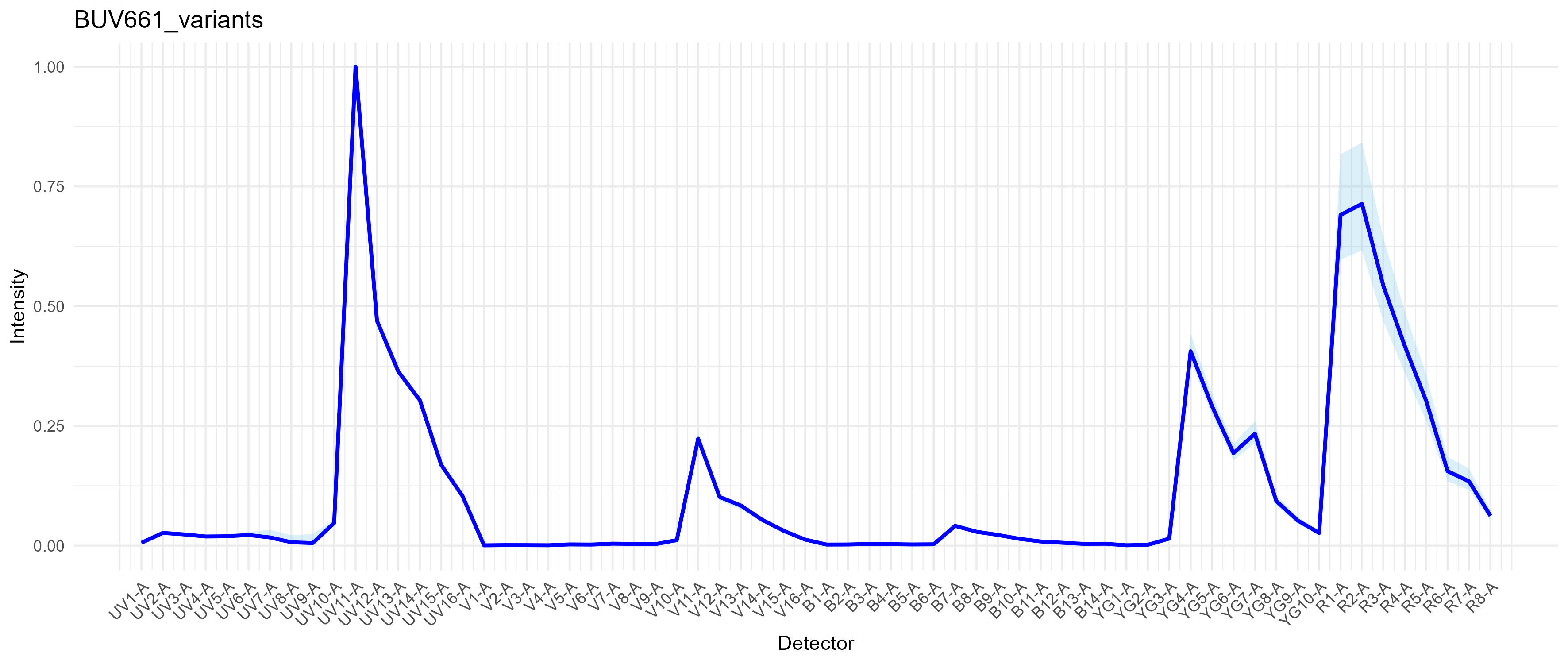The dark blue trace is the optimized single spectrum from spectra. The light blue region represents the range of variation across all the variant spectra. Specifically, the min and max for each channel are being plotted.

Notice that the main variation is in the R1 and R2 detectors, indicative of variation in the direct excitation of the red laser-excited acceptor molecule in BUV661. It’s hard to get good information about the structure of the Brilliant dyes, but they’re long polymers and all except for the shortest emission ones (e.g., BUV395, BV421, BB515 and also BV510) are tandem dyes. BUV661 is probably a tandem of BUV395 and something like Cy5. So, what we are seeing is variation in the ratio of direct Cy5 excitation by the 561nm laser to excitation of BUV395 by the 355nm laser. There are a lot of reasons why this could be happening. One explanation that I consider to be likely is that we have a distribution of species of BUV661 in the conjugated antibody, either due to production variation (not so likely) or tandem breakdown (more likely). When we stain our cells, the distribution of conjugates on any given cell will give a certain result (think of 80 intact molecules and 20 somewhat broken ones on cell A, and perhaps 85:15 on cell B), which will result in a distribution at the population level. There’s also electronic noise and measurement error in the mix. Anyway, we get some cells with more red emission and some with less, which will create variability in amount of red signal from BUV661. This means that if we put a fluorophore in our unmixing that uses R1 and/or R2 heavily, say APC, we will observe variability in the cells that are positive for BUV661 with respect to APC. Hence, spillover spread. There are some broader implications here for panel design and other issues in the field, I think.

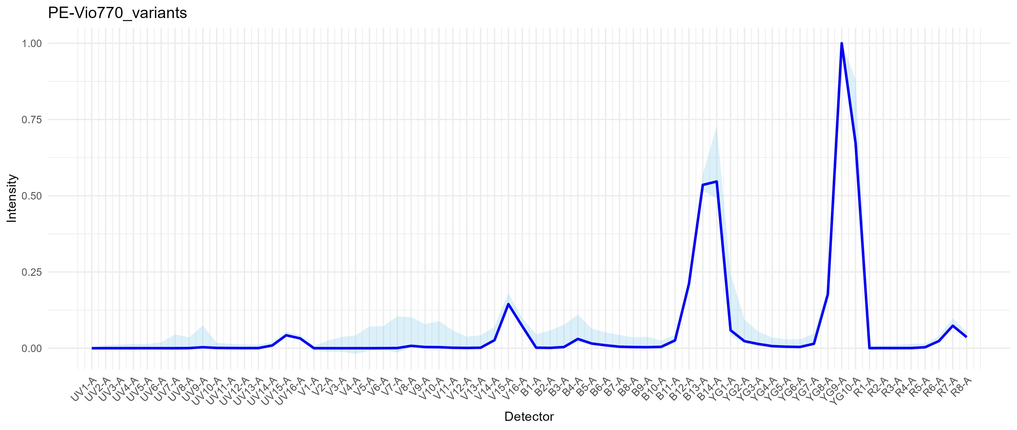
Here’s PE-Vio770 (anti-ACSA-2), which is essentially PE-Cy7. See that there’s a wide light blue region around YG1, which is where the base donor PE molecule emits. This means we have some tandem breakdown and that there is a range of species in the vial. The variation in the mid-UV, mid-violet and narrow-blue is AF.

PE-Vio770 variation

Okay, now we’re ready to unmix with per-cell fluorophore optimization.

This is where we start Tetrising.

We are going to try to figure out which of these variants is the best “fit” for each cell in the data. We do this by trying to fill in the little gaps, the mismatch, in between the raw data and the prediction from the unmixing model. This gap is call the residual, which is the part of the data that cannot be explained by the model. We want the model to be as good as possible, which means minimizing that gap. One way of thinking of the unmixing is that we are trying to squeeze the spectra into the raw data. We can multiply them up and down to scale them, but we don’t normally get to change the shapes at all. With the variants, we have options, all of which are very, very similar, but that small flex allows us to fit the shapes in better.

The most accurate way of doing this would be to test not only each variant for each cell, but to test each combination of variants, probably in an iterative refinement. Since that would increase at the rate of n.variants^n.fluorophores, it is currently prohibitive to do so. Note that this does not even begin to deal with variation outside the range of what is seen in the single-stained controls. Up to version 1.0.0, AutoSpectral has used a “brute force” approach of testing every variant for every cell, at least for the “slow” method. This is indeed slow.

As of version 1.0.0, we speed up the process by pre-screening variants per cell. We can do this by looking for variants where the change in the spectrum between the variant and the base/median spectrum for that fluorophore matches the shape of the residuals for the cell. Basically, we are looking for alignment or similarity between what the change in spectrum will do and what the cell has “left over”. This means we’re only looking for variation that pushes in the “correct” direction. By doing this, we can cut down to a handful of potential candidates (or even a single one) rather than testing a hundred or so per fluorophore. That allows us to speed things up a lot, without affecting the results much at all. In some cases, this gives a slightly better result since we don’t get trapped in local minima. Since we are no longer testing every variant for every cell, we can pass a larger set of variants without affecting the computation time much at all, and AutoSpectral offers that in version 1.0.0. This can help slightly, but tends to be less important than screening more autofluorescence spectra.

Anyway, running this in pure R is now possible, albeit slow. The faster implementation is in C++ and requires installation of AutoSpectralRcpp. I strongly encourage you to install that prior to running unmixing as below. Also, be sure that you have the fast BLAS and LAPACK installed. Please reach out if you have suggestions for faster implementation (I’m not a computer scientist). See the article on Computing Speed for full tips.

As of version 1.6.0, there is a change to how the variants are evaluated. Up to this point, selection of the best variants has been done in a reduced fluorophore space, using on the fluorophores that are “positive”, i.e., above the unstained threshold, in a given cell. This is faster, since we aren’t solving for everything all the time, and gives us a residual that is more informative (we effectively have a smaller panel for each cell, so any leftover bits are easier to assign). That trick is responsible for the appearance of discontinuities in the unmixing, though. So, version 1.6.0 uses a different approach involving the covariance matrix, which looks at the pattern of variation we are seeing for the spectrum of a given fluorophore and asks how it is likely to propagate into the unmixed data as error or spread. This allows us to know more or less where we are going to get error. The residual then, ideally, tells us the direction of the error. Additionally, this approach holds off on committing to a variant for a fluorophore until any other fluorophores that are competing for that same bit of information have also been assessed. Because of this, we can often get a bit better solution (better unmixing), but it may take longer, and may require multiple rounds or “passes” to achieve the best result.

So, the covariance approach is now the default option for unmixing when you supply variant information. If you want to use the original method for consistency, it is still available. Just specify pipeline = "legacy".

fully.stained.dir <- "./Fully stained"

unmix.fcs( fcs.file = file.path( fully.stained.dir, "C3 Lung_GFP_003_Samples.fcs" ),
           spectra = spectra,
           asp = asp,
           flow.control = flow.control,
           method = "AutoSpectral",
           af.spectra = lung.af,
           spectra.variants = variants,
           parellel = TRUE,
           threads = 0,
           pipeline = "joint",
           n.passes = 1 )

Most datasets I have tested show good results with a single pass. Setting n.passes to anywhere between 2 and 10 can show some improvement, larger improvement in some messy data sets. This will increase the computational time roughly linearly unless the data converges early.

Additional joint-pipeline tuning

A few more arguments let you tune the joint pipeline beyond n.passes:

Multipass autofluorescence refinement. n.af.passes (default 1) controls how many AF extraction passes are run per cell. The first pass uses matching pursuit to assign an AF candidate to every cell; if n.af.passes is greater than 1, subsequent passes revisit the highest-abundance AF cells (controlled by refine.af.quantile, default 0.5, the fraction of cells taken forward for reassessment — set to 1 to reassess everyone) and can refine the AF assignment further. Like n.passes, this trades additional computation time for improved AF characterization, and is most useful for tissue samples with more heterogeneous autofluorescence; PBMC data typically shows negligible benefit.

Collinear fluorophore handling. collinear.threshold (default 0.5) sets the cosine similarity above which two fluorophore variants are treated as structurally collinear (e.g. APC/BUV661) and routed into conflict resolution rather than independent assignment. Lower values trigger conflict resolution more often (more thorough, slower); higher values allow more variants to be committed based on minimizing spillover from the brighter fluorophore alone, which is faster but can understate a dimmer collinear fluorophore’s true abundance. joint.pair.resolution (default TRUE) turns this conflict-resolution step on or off; when enabled, a small combinatorial test is run specifically for the competing pair(s) to find a better joint solution.

Per-cell detector weighting. cell.weight (default FALSE, but TRUE automatically on ID7000 data) applies per-cell weighting to the joint solve based on each detector’s fitted signal, with noise.floor (default 125) preventing near-dark channels from receiving runaway weight. alpha (default 0.5) balances residual minimization against covariance-based spillover minimization when scoring candidate variants.

Most users won’t need to touch these — the defaults were chosen from testing across Aurora, ID7000 and S8 data — but they’re there if you’re working with an unusually noisy panel or you want to explore how they impact the unmixing.

Unmixed FCS files will appear in folder ./autospectral_unmixed.

Add a file.suffix argument if you want a tag on the FCS file’s name to differentiate it from other versions.

Legacy pipeline notes:

Setting the “speed” determines how many pre-screened candidate variants will be tested per cell. The options are “fast” = 1, “medium” = 3, and “slow” = 10. This is based on quite a bit of testing with high parameter data from the Aurora, ID7000 and S8. For data with messier fluorophores (like that BUV661 above), using “slow” is likely to show some improvement. If you are using more modern fluorophores, you may find minimal difference now when using “fast”.

If you want to set the number of variants yourself, you can do this by providing the n.variants argument. This will override “speed”. In the call below, for instance, we’ve requested to test up to 100 variants per cell (depending on what’s actually available). This would be comparable to the previous “slow” brute force approach.

unmix.fcs( fcs.file = file.path( fully.stained.dir, "C3 Lung_GFP_003_Samples.fcs" ),
           spectra = spectra,
           asp = asp,
           flow.control = flow.control,
           method = "AutoSpectral",
           af.spectra = lung.af,
           spectra.variants = variants,
           n.variants = 100 )

Accuracy

To demonstrate the effectiveness and accuracy of this approach, we created a set of synthetic data. In this 42-colour data set from the Aurora, BUV661 and APC are used to detect CD19 and Foxp3, markers that are not co-expressed. We created a set of data in silico where the raw data for BUV661+ and APC+ events (based on OLS unmixing) were combined or maintained as separate original events. In this way, ground truth is available for BUV661+, APC+ and BUV661+APC+ events. When unmixed using OLS, populations containing BUV661 suffered from misclassification with respect to a positivity threshold for APC set based on a value double that of the 99.5th percentile on the unstained sample. These false positivity errors were reduced when per-cell spectral selection was performed, and the median absolute deviation of ground truth BUV661+APC- events in the APC channel was reduced from 2194 to 723.

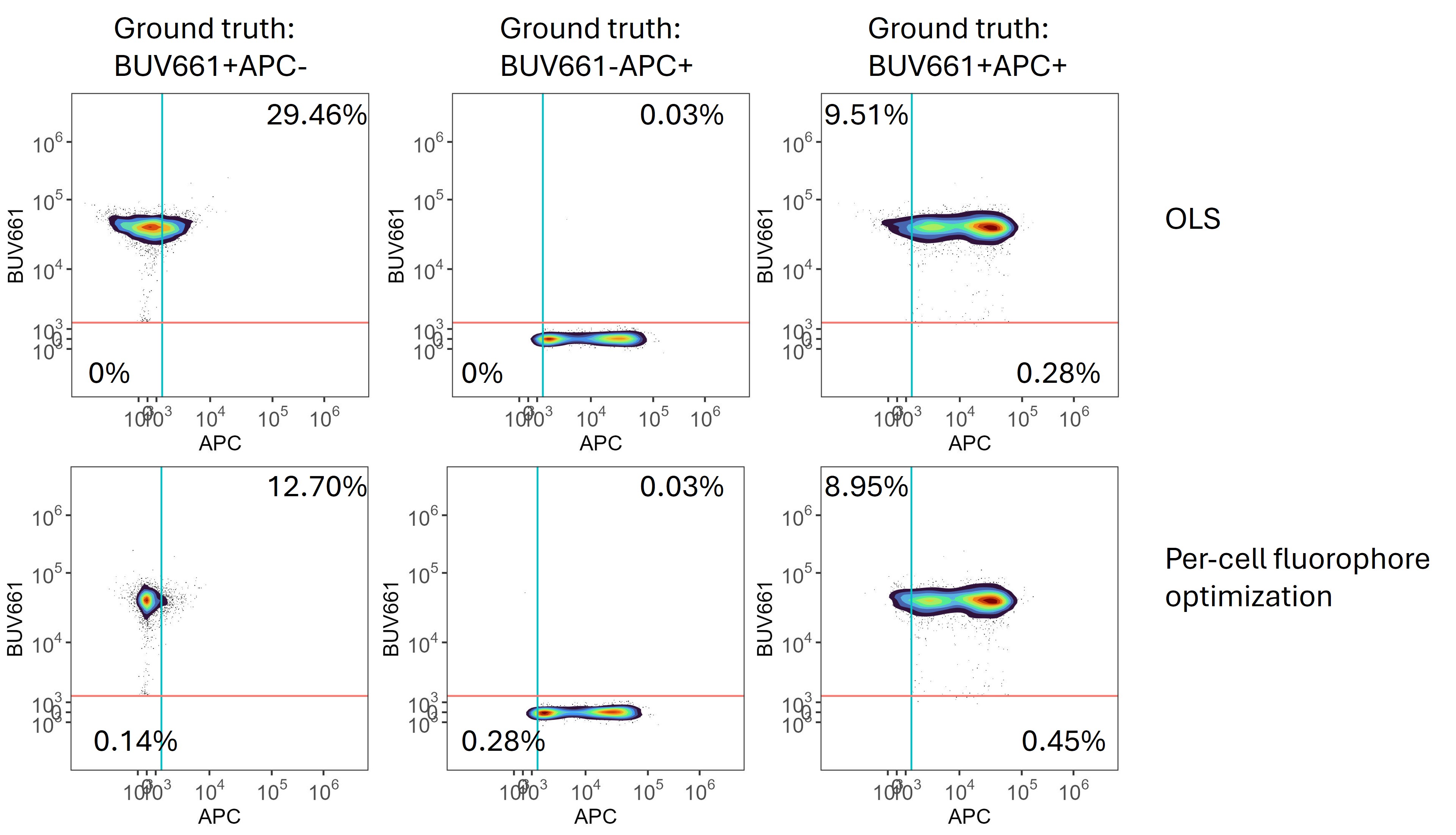Synthetic data showing that per-cell optimization of the fluorophore signatures reduces spillover spread. This example was produced using the legacy pipeline. Similar results are obtained with the new joint covariance pipeline.

Correspondingly, the cosine similarity between the model’s predictions for BUV661 and the actual data for BUV661 was closer to 1 (identity), consistent with more accurate modelling of the underlying data.

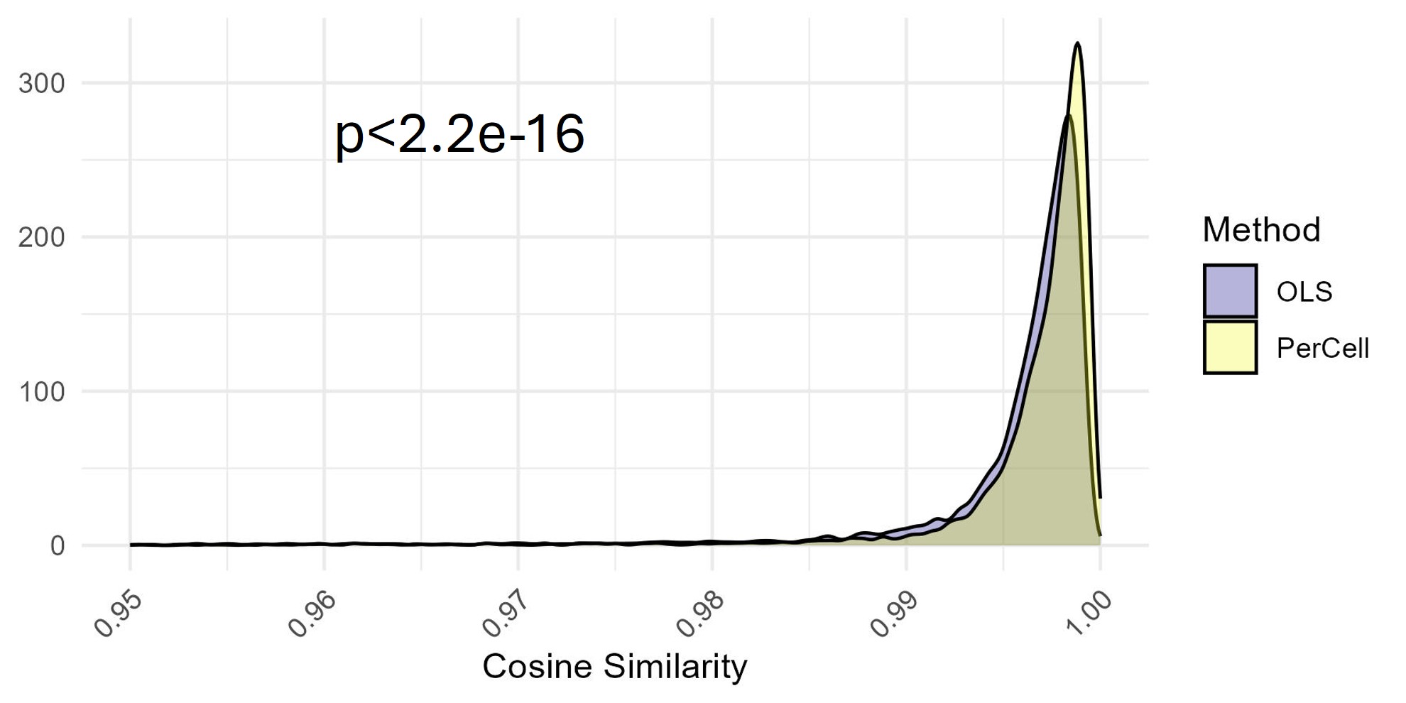Distribution of cosine similarity values between the ground truth and the assigned spectrum for BUV661. Comparison between standard OLS unmixing and AutoSpectral with per-cell fluorophore optimization on synthetic data. Stats by Komogorov-Smirnov test.