10 Single Cell Autofluorescence • AutoSpectral

The aim of this article is to show you how to use AutoSpectral’s per-cell autofluorescence (AF) extraction. This method selects the best AF signature to use for each cell (or point of debris, noise, whatever) in the data.

The first thing we need to do is discover all of the AF signatures present in the data. For this, the unstained control is critical. For good results, you need to do the following in your wet lab work:

Prepare a truly unstained sample. This means no added fluorophores, so no conjugated antibodies or live/dead stains and no fluorescent buffers such as the Brilliant Stain buffer. This also means no fluorescent reporters. If you run GFP expressing cells as your unstained, the GFP signal in those will be considered an AF signature, and it will be unmixed as autofluorescence rather than GFP. If you contaminate your unstained with small amounts of stained cells, single-stained controls or fluorescent beads, those signatures may also be considered to be AF.
Treat your unstained sample like your fully stained sample. Run it through the same protocol. If you’re fixing and permeabilizing, do that to the unstained, too. * 3) Acquire lots of cells. If you only acquire 10 thousand events, you will have very little data to work with, and rare populations, which are probably the problematic ones, will not show up well. Ideally, run as many cells as in your fully stained samples.
Run unstained samples for each sample type in your data if you expect a difference in AF For example, with tissue samples, run a sample from spleen, lymph nodes and lung, not just spleen or lung. If you’re running samples from drastically different conditions (e.g., infected vs. healthy or infant vs. adult), I suggest running an unstained for each.
For smaller differences in conditions, you will probably get good results by creating a pooled unstained sample. For instance, when running PBMC from multiple donors, you could take a few cells from each for the unstained sample for AF.

You’re welcome to play around with breaking these rules to see what happens.

A note about pooling: This can be done in the wet lab by mixing the cells into a single tube. A safer, and likely more representative option is to mix in silico after acquisition. This can be done by concatenating the FCS files or by using a function such as AggregateFlowFrame() from FlowSOM. There is now a concatenation function available directly in AutoSpectral, which you can access via concatenateFCS().

library( AutoSpectral )
#> AutoSpectralRcpp detected: using Rcpp-accelerated readFCS and writeFCS.

Before doing the single-cell AF extraction, you’ll need to either run the AutoSpectral workflow to extract your fluorescence spectra or extract the spectra using another method (e.g., FlowJo or from the Cytek .Expt file). This is because we will use these spectra in the determination of the AF spectra. We’re going to be looking at both the raw and unmixed versions of the unstained sample in order to determine how the AF signatures present are likely to interfere with the unmixing.

asp <- get.autospectral.param( cytometer = "aurora", figures = TRUE )
control.dir <- "./SSC"
control.file <- "fcs_control_file.csv"
flow.control <- reload.flow.control( control.dir, control.file, asp )
spectra <- get.spectra.automated( control.dir, control.file, asp )

Now we are ready to get the AF spectra. For this data set, we have spleen, lung and brain samples from mouse. We can do all three. I’ve got the files in the ./SSC folder, but be sure to pass the file path as well as the file name to the first argument of get.af.spectra.

unstained.lung <- "G2 WT Lung_Samples.fcs"
unstained.brain <- "G3 WT Brain_Samples.fcs"
unstained.spleen <- "G1 WT Spleen_Samples.fcs"

lung.af <- get.af.spectra( file.path( control.dir, unstained.lung ),
                           asp, spectra, title = "Lung AF" )
brain.af <- get.af.spectra( file.path( control.dir, unstained.brain ), 
                            asp, spectra, title = "Brain AF" )
spleen.af <- get.af.spectra( file.path( control.dir, unstained.spleen ), 
                             asp, spectra, title = "Spleen AF" )

This call reads the FCS file, unmixes it, and creates a self-organizing map (SOM) of the combined raw and unmixed data. Each SOM node (map$code) is considered an AF signature. Note that you can increase or decrease the number of spectra generated by changing the SOM dimensions with argument som.dim. The default 10 generates 100 spectra (10 x 10), which works quite well. It’s likely overkill for simple AF mixtures like PBMCs, but it does not hurt except for taking longer during the unmixing. If you have really messy samples, you could play around with larger SOMs, but the default settings work well for mouse lung, which is pretty terrible for AF.

If you feel that the number of AF spectra being generated is overkill, you can reduce the number by deduplicating similar spectral profile. This can be accessed through the logical parameter deduplicate (default is FALSE) and the cosine similarity threshold controlled by deduplication.threshold = 0.99. In testing, deduplication reduces the accuracy of per-cell AF assignment, as should be expected, but the impact is minor.

Before the SOM is even built, get.af.spectra() also screens the unstained sample itself for likely contamination. Any event whose cosine similarity to a fluorophore spectrum in spectra meets or exceeds contaminant.threshold (default 0.99) is removed prior to clustering; this is controlled by the logical remove.contaminants (default TRUE). This per-event check is more sensitive than a post-hoc check on the finished AF spectra, since a handful of contaminating events (a stray stained cell, a bead) are unlikely to dominate an entire SOM node on their own, but would otherwise get baked into an AF signature.

We get output plots of the AF signatures in the figure_autofluorescence folder.

Lung AF Lung AF Lung AF

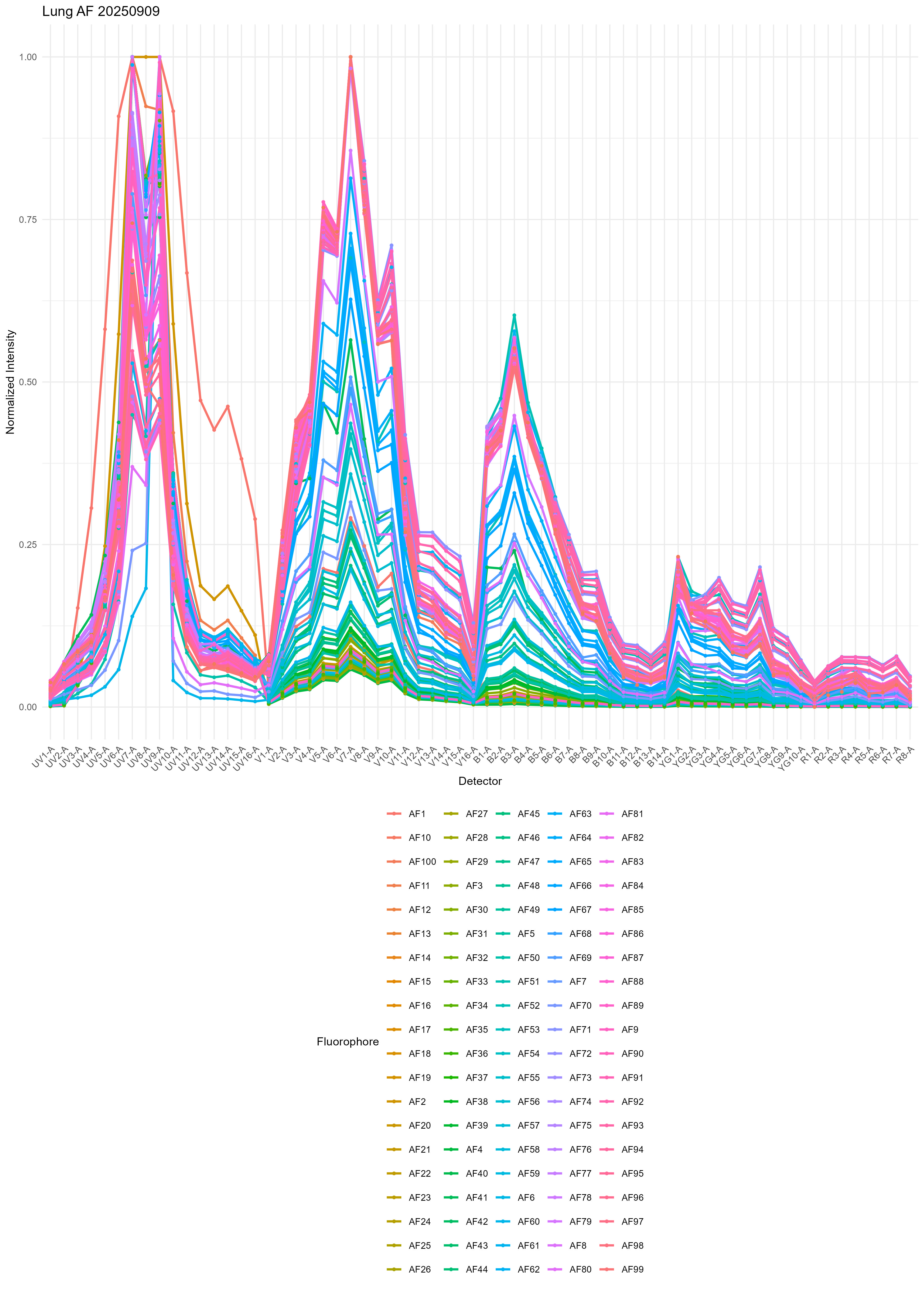
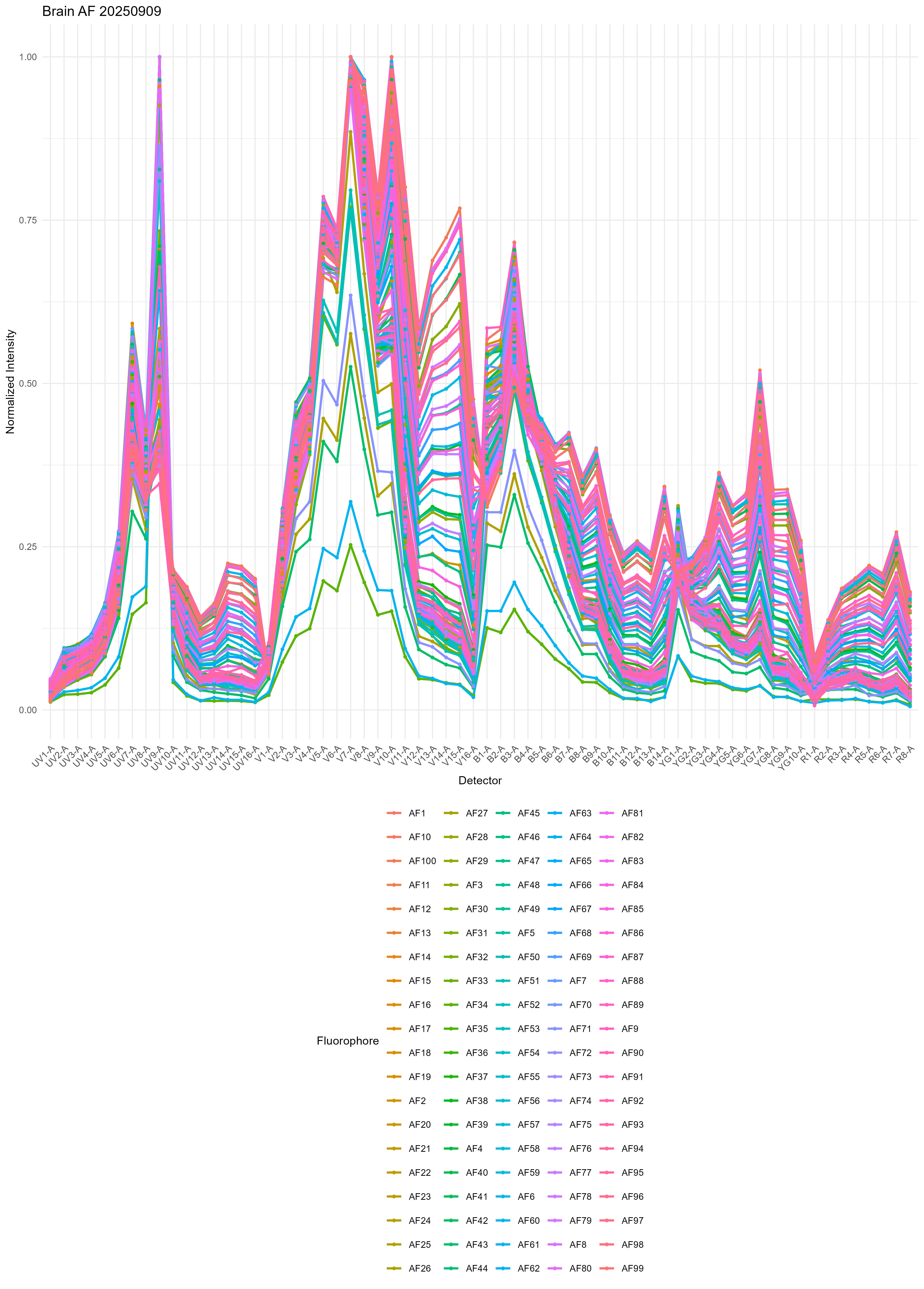
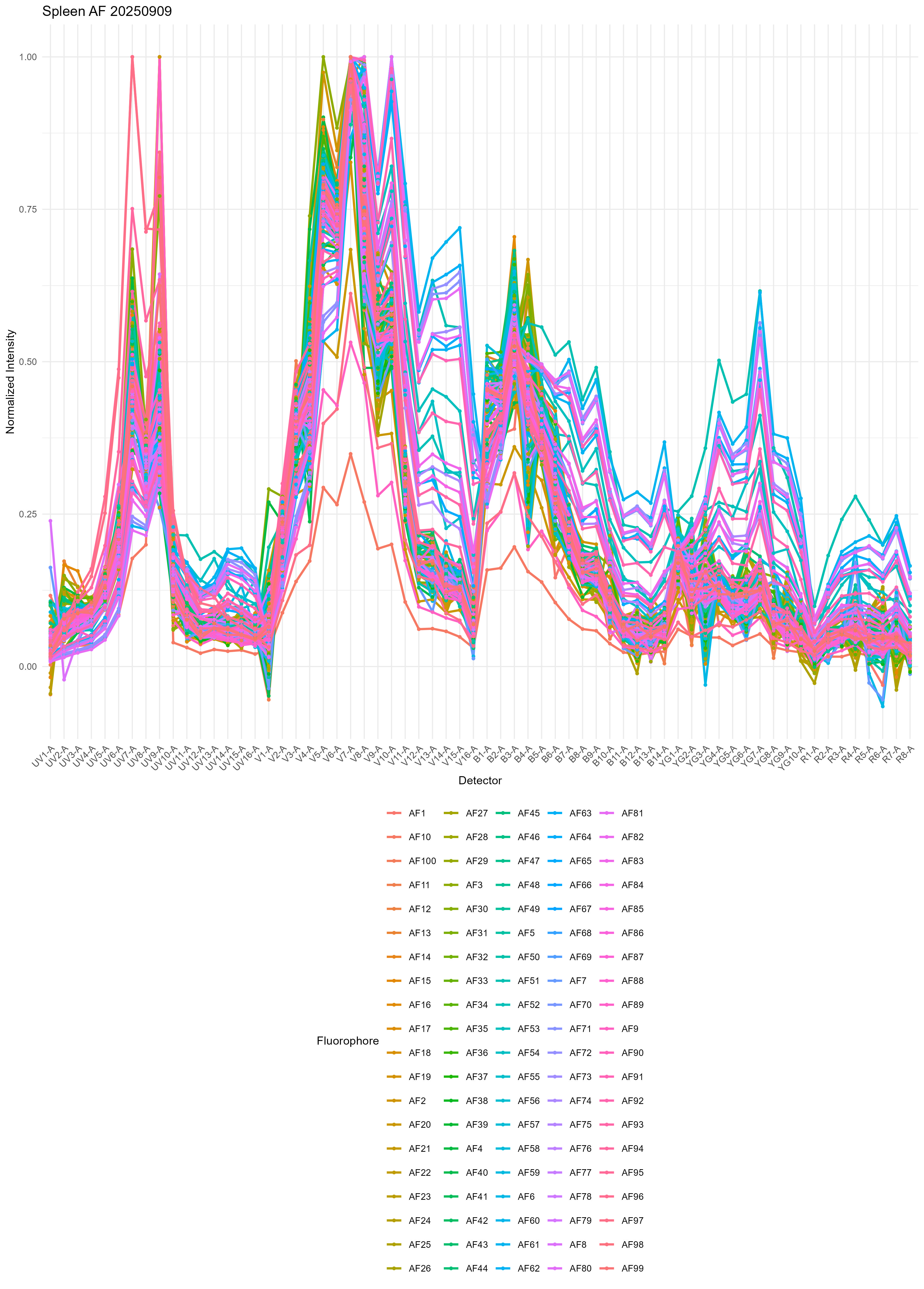
From the variability, I think you can start to understand why it’s really hard to get good results with single or multiple AF extraction using the standard method.

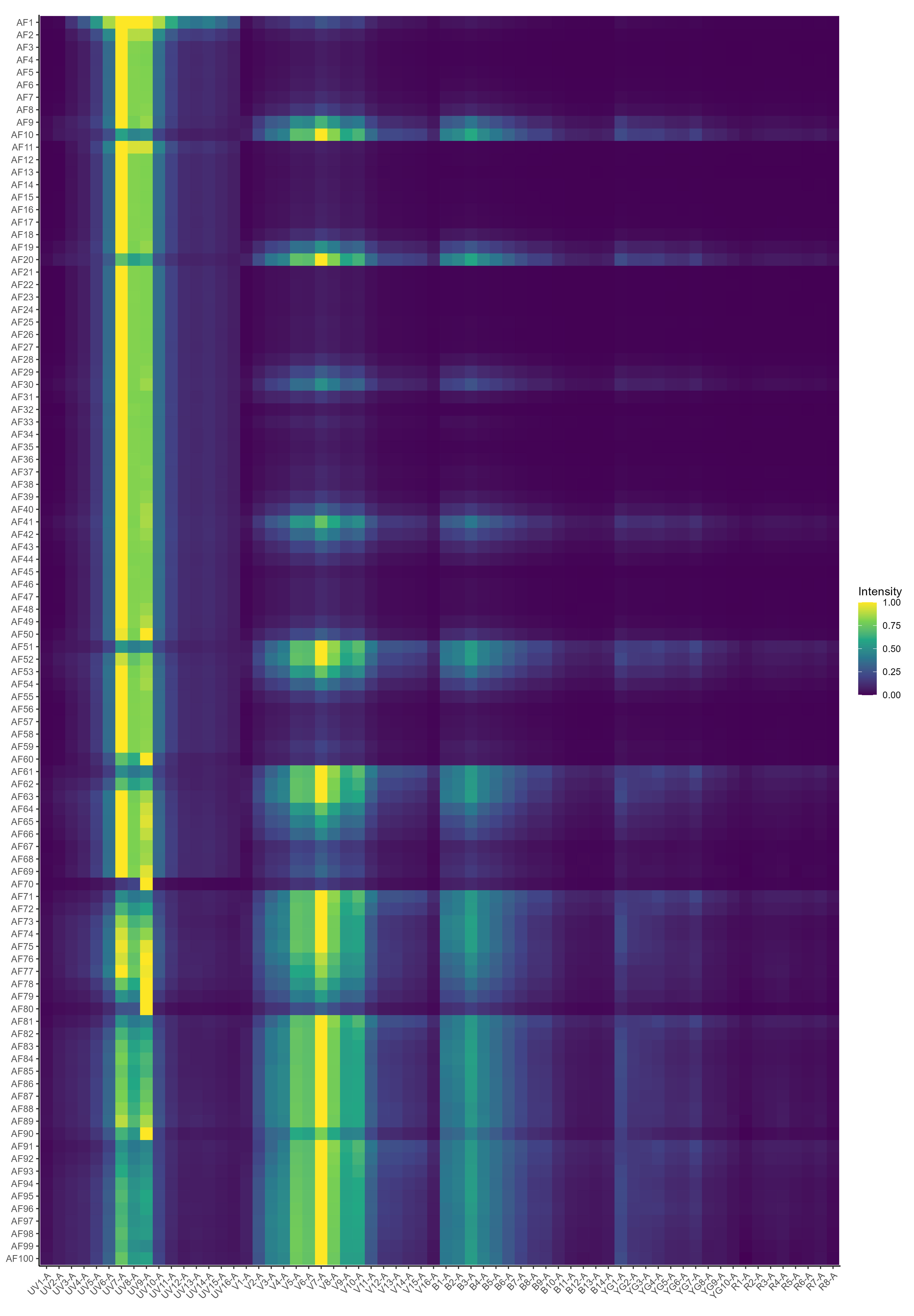
There’s also a heatmap generated, but I don’t find this so useful. If you want, you can probably create some nicer looking plots with some metaclustering or a dendrogram to group the AF signatures. We don’t use metaclustering on the SOM nodes because this gives slightly inferior results in the unmixing.

Lung AF heatmap

Okay, now we’re ready to unmix with per-cell AF extraction.

If you are working with multiple sources like in this example, be sure to provide the corresponding AF for the unmixing. For example, for lung cells, provide the lung AF spectra. If you provide a non-matching AF, it won’t create problems (based on both theory and empirical testing), but the results will not be as good as if a matching one were used, simply because the best match won’t be present for all cells. Note that this means you can use pooled samples as long as you have enough events acquired, although you may need to increase som.dim or set refine=TRUE if there are a lot of AF signatures present in each part of the pool.

Refining the AF spectrum library (Version 1.0.0)

Version 1.0.0 changes the way autofluorescence spectra are identified slightly, allowing for a second round of identification of cells that are likely to be problematic given only the first set of AF spectra. This is done by using AutoSpectral’s per-cell autofluorescence extraction on the unstained sample. Any signal in the fluorophore channels in the unmixed unstained data can be considered to be error. In the update, we select the cells that are the furthest from zero in the unmixed space and run a second round of clustering on these, updating the AF spectra that were used to unmix them. This expands the set of possibilities, focusing on the worst offenders. This is most useful for complex tissue samples, and allows extraction of the problematic last 1-3% of cells that are in the wrong place. To use this expanded set, run get.af.spectra() with refine=TRUE. Note that refine = TRUE is the default as of version 1.0.0.

Note that this is distinct from the multipass AF assignment option described later in this article (n.af.passes). This section is about building a better library of AF spectra before unmixing ever happens; n.af.passes is about giving each cell more than one shot at matching against that library during unmixing itself.

Extracting AF for each cell

While you can call unmix.autospectral() or unmix.autospectral.rcpp() directly, this requires reading in the FCS file into R, extracting the expression data and so on. The better option is to just call unmix.fcs directly, which will create an unmixed FCS file from your raw FCS file.

fully.stained.dir <- "./Fully stained"

unmix.fcs( fcs.file = file.path( fully.stained.dir, "C3 Lung_GFP_003_Samples.fcs" ),
           spectra = spectra,
           asp = asp,
           flow.control = flow.control,
           method = "AutoSpectral",
           af.spectra = lung.af )

Unmixed FCS files will appear in folder ./autospectral_unmixed.

Multipass AF assignment for complex samples

For particularly messy samples (tissues, tumors), a single AF subtraction pass per cell may not remove everything it should, particularly for the higher-abundance “worst offender” cells. The joint unmixing pipeline underlying unmix.fcs() (see unmix.autospectral.rcpp(), backed by unmix_autospectral_joint_pipeline.cpp) supports a second pass of AF assignment, on top of whatever spectra you generated with get.af.spectra().

This is controlled by two arguments to unmix.fcs():

n.af.passes (default 1L): the number of AF assignment passes to run per cell. Setting this to 2 re-scores the residual left over after the first pass against the AF library and, if a better match is found, adds that AF contribution on top of the first pass’s estimate.
refine.af.quantile (default 0.5): controls which cells are taken forward for the additional pass(es). Only cells at or above this quantile of first-pass AF abundance are re-scored; the rest are left as-is. Set to 1 to force every cell through additional passes, though this is rarely necessary and will increase unmixing time. Testing suggests that a value of around 0.7 will be good for most problematic samples, so 0.5 is generous.

unmix.fcs( fcs.file = file.path( fully.stained.dir, "C3 Lung_GFP_003_Samples.fcs" ),
           spectra = spectra,
           asp = asp,
           flow.control = flow.control,
           method = "AutoSpectral",
           af.spectra = lung.af,
           n.af.passes = 2L,
           refine.af.quantile = 0.5 )

As with get.af.spectra(refine = TRUE), this is aimed at complex AF samples and comes at some cost in processing time proportional to the fraction of cells re-scored. For clean PBMC-type samples, the default n.af.passes = 1 is usually sufficient.

unmix.fcs() also exposes several other joint-pipeline tuning parameters (cell.weight, alpha, collinear.threshold, joint.pair.resolution, noise.floor) that control the per-cell fluorophore variant optimisation rather than AF extraction; see ?unmix.fcs for details.

Go Faster

Per-cell AF extraction involves a lot of unmixing. Visit the article on Speed for tips on setting up your computer for faster processing.

As of version 1.0.0, the process of assigning AF signatures to individual cells (and then unmixing them) has been sped up in C++. Processing time is now comparable to standard unmixing. For this, you will need to install AutoSpectralRcpp.