Full Workflow Example

Installation

If you need to install AutoSpectral, run this bit first:

# Install Bioconductor packages
if (!requireNamespace("BiocManager", quietly = TRUE))
  install.packages("BiocManager")
BiocManager::install(c("flowWorkspace", "flowCore", "PeacoQC"))

# You'll need devtools or remotes to install from GitHub.
install.packages("devtools")
devtools::install_github("DrCytometer/AutoSpectral")

Get the data

Download the data for today’s example from Mendeley Data.

These data are a 9-colour panel run on a 5-laser Cytek Aurora. The samples are from spleen, lung and liver. This is a pretty simple experiment, which is nice since it will run quickly. The different tissues allow us to look at how to handle diverse autofluorescence profiles. I’ll point out that this panel has been deliberately designed to accommodate autofluorescence peaks, so we can expect autofluorescence removal to work pretty well with any method. In my testing, you can use multiple autofluorescences and get good results; you can also use deconvolution of the autofluorescence using principal components. Both produce good results with a highly over-determined data set like this. We’ll look at the per-cell autofluorescence extraction with these data, which has the advantage of also working on large panels.

Start-up

Now we can load AutoSpectral.

library(AutoSpectral)

Getting your fluorophore spectra from the controls

Since the default cytometer is the Aurora, we can actually just call this without any arguments. Otherwise you need to specify the cytometer you’re using.

asp <- get.autospectral.param()

Where are the controls? This must be typed correctly.

control.dir <- "./Raw/Set1/Reference Group"

Create the control file. You will need to manually edit your control file, telling AutoSpectral what’s going on. It will try to fill in some stuff for you, but you should check this. See the article on this on GitHub or Colibri Cytometry.

create.control.file(control.dir, asp)

We get warnings because I’ve got both bead and cell controls, and AutoSpectral would like me to pick one per fluorophore. This isn’t strictly necessary, so if you want to bypass this, just change the names in the “fluorophore” column of the control file to be unique names. For instance, you could have “PE cells” and “PE beads”. Note, however, that whatever you put as the “fluorophore” is what gets written to the description of the channel in the FCS file later on. So, you’ll be better off picking one control per fluorophore. If you have a situation like this, you can run the controls in different flow.control sets, figure out which you like best, and then do a final version with the best choices.

Here’s what the control file looks like as first generated: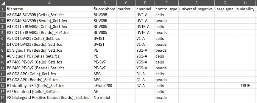

Here’s what we want it to look like: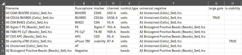

For more on this, see the Control File article on GitHub.

Once you’ve got it the way you want, write in the name of the control file and run the error checking function.

control.file <- "fcs_control_file.csv"
check.control.file(control.dir, control.file, asp)

Once, the control file passes the error checks, we can load in the data. This part can be a bit slow, particularly if you have lots of big files. There is a parallelization option, which can cut the time in half, probably even better on Mac/Linux. There are some improvements I could make to this, including the gating. These will take time to implement, though, because they affect everything downstream of this, which is to say, everything.

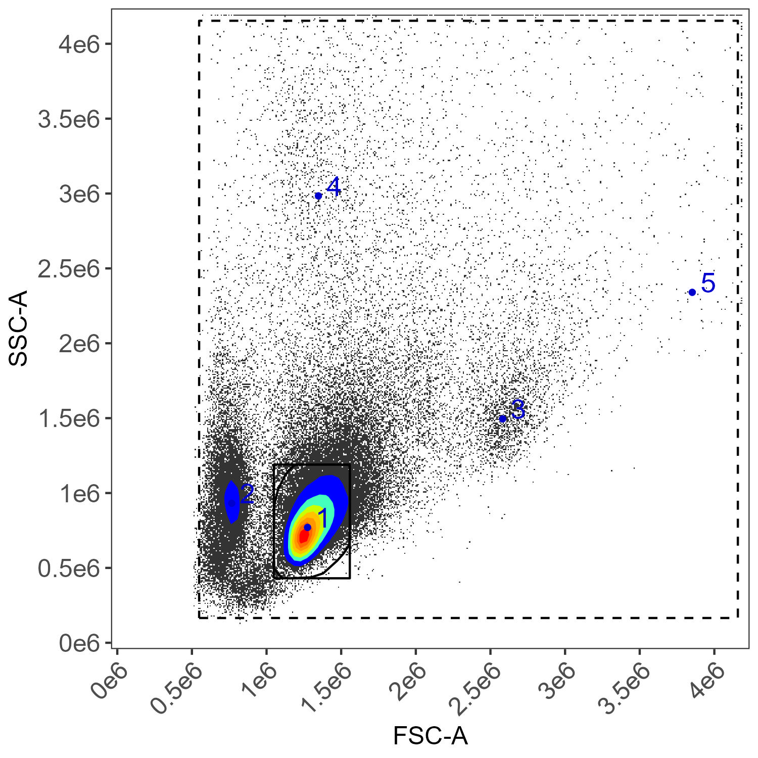
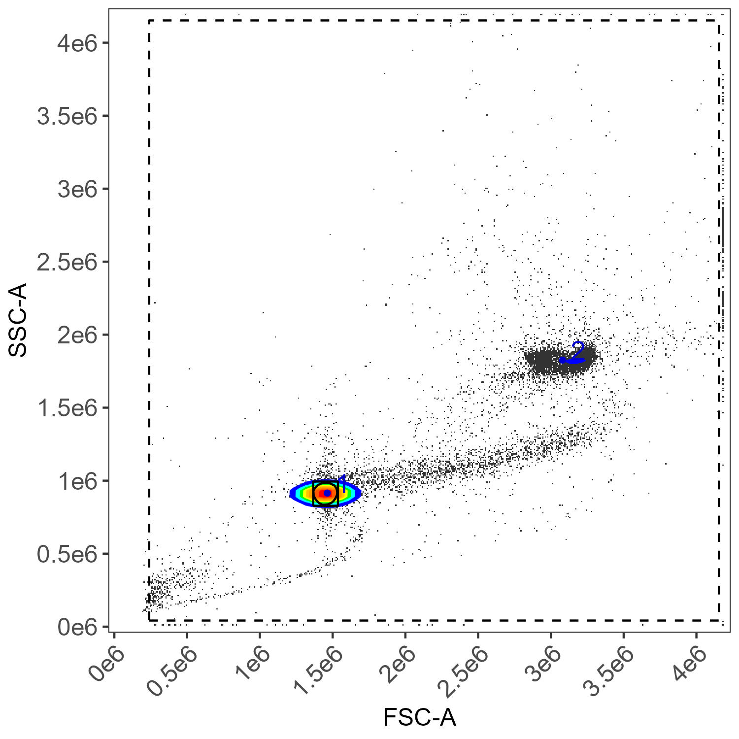
flow.control <- define.flow.control(control.dir, control.file, asp)

Be sure to check the gates that are generated in the figure_gate folder–do they look right? If not, go to the Gating article on GitHub/Colibri for tips on how fix it.

Cell Gate

Bead Gate

If everything looks okay with the gating, we proceed to control clean-up. This helps remove noisy events, like autofluorescence spikes, and tries to match the positive events for each control to corresponding cells/beads in the unstained universal.negative that you defined in the control.file.

The default settings here are usually best. There is a parallelization option, which is being converted to the new parallel backend. Once that is in place, it should be faster.

flow.control <- clean.controls(flow.control, asp)

There are lots of plots generated with this, in figure_clean_controls and in figure_spectral_ribbon.

Now we can isolate the spectra from the controls. By default, this uses the cleaned data if they are available.

spectra <- get.fluorophore.spectra(flow.control, asp)

With this, we get plots of the spectra as traces and a heatmap. We also get a cosine similarity heatmap. You can check these, if you aren’t familiar with what they should look like, against the expected profiles in online webtools. For the Aurora, check on Cytek Cloud.

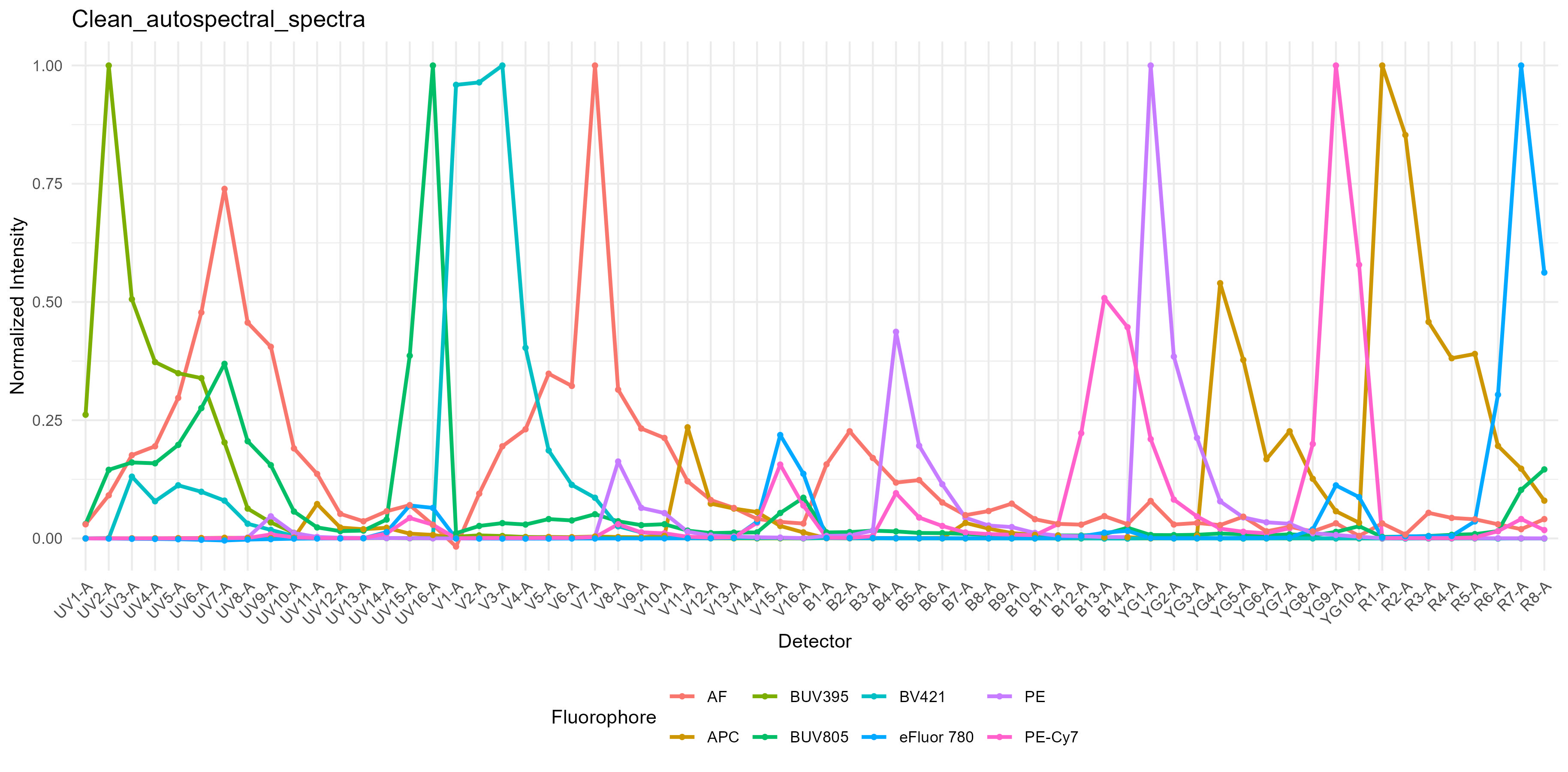
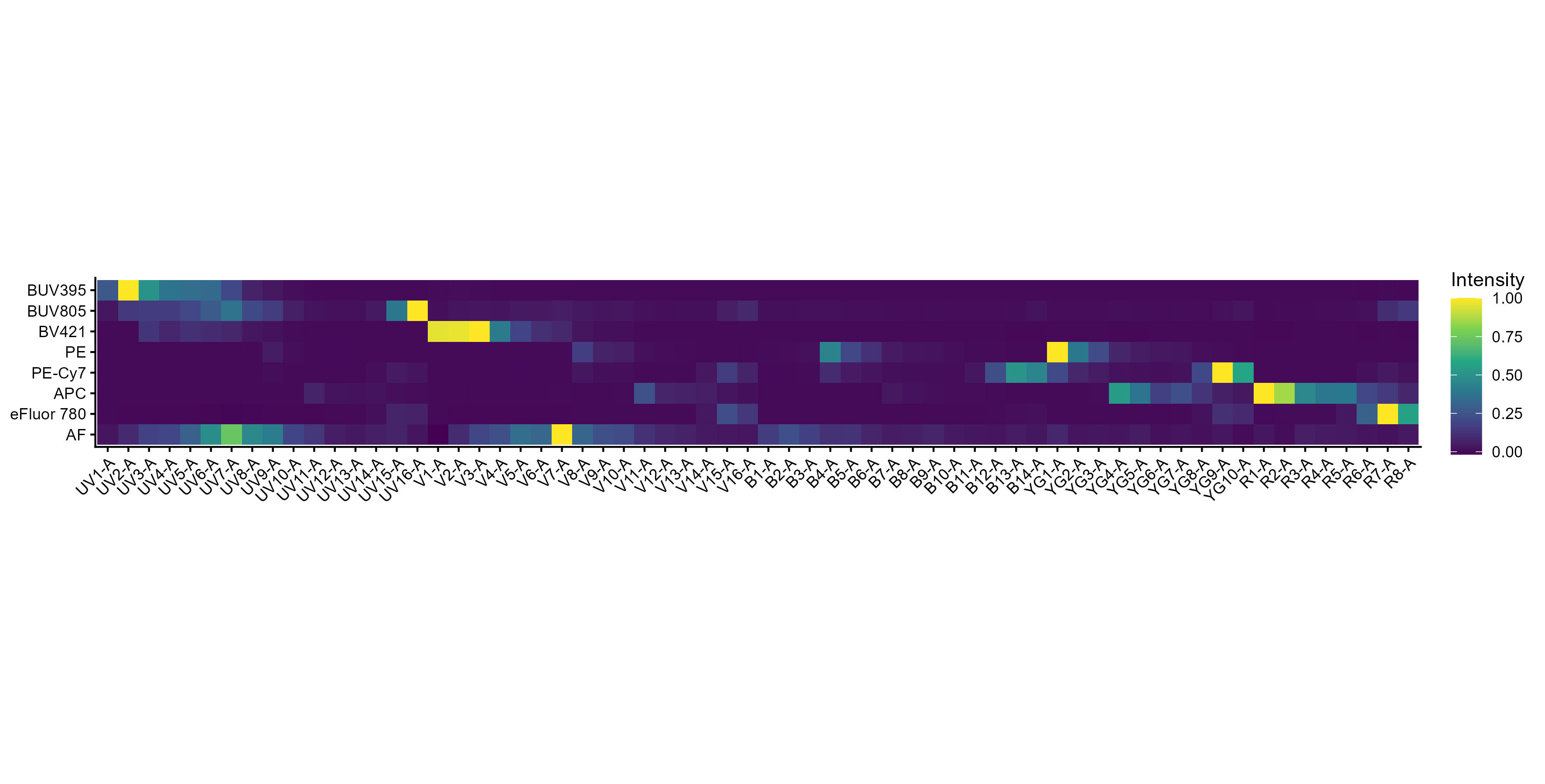
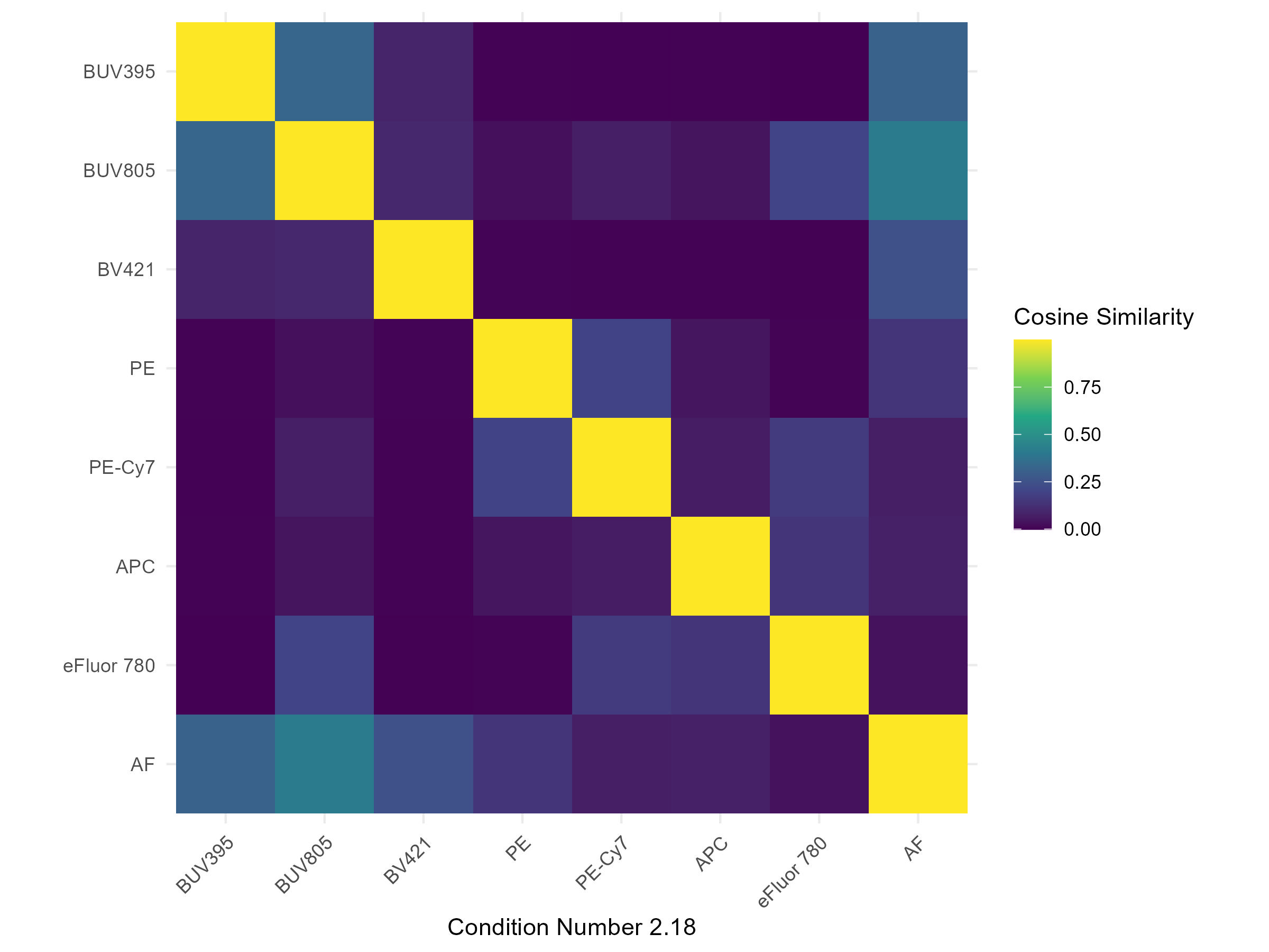
The spectra themselves are saved to a CSV file in the table_spectra folder. You can open CSV files as a spreadsheet in Excel and other programs.

Now, on to unmixing.

AutoSpectral provides options for unmixing. Let’s start with the most basic, which is replicating the OLS unmixing as in SpectroFlo. Autofluorescence extraction with OLS and WLS unmixing in AutoSpectral is handled by including an “AF” signature in spectra. This is generated automatically from the unstained cell control sample that is tagged as “AF” in your control.file. We can use OLS or WLS without autofluorescence extraction by removing this row from the spectra matrix before we pass it to the unmixing call. Here are two easy ways to do that: 1) subset spectra 2) read in the CSV file in table_spectra, removing the AF channel

rownames(spectra)
no.af.spectra <- spectra[ !(rownames(spectra) == "AF"),]
rownames(no.af.spectra)
no.af.spectra.2 <- read.spectra("Clean_autospectral_spectra.csv",
                                remove.af = TRUE)
rownames(no.af.spectra.2)

To unmix, specify the file (and path) of the FCS file you want to unmix:

spleen.fcs.file <- "./Raw/Set1/Stained/D4 Spleen_Set1.fcs"
unmix.fcs(spleen.fcs.file, spectra, asp, flow.control,
          method = "OLS", file.suffix = "with AF extraction")
unmix.fcs(spleen.fcs.file, no.af.spectra, asp, flow.control,
          method = "OLS", file.suffix = "without AF extraction")

If we have a folder full of FCS files, we can do all the files in the folder. Note that this is essentially just an lapply loop over the files. It can, however, be parallelized, which will work as long as you have enough memory to handle the number of threads multiplied by the size of the files. So, if your FCS files are ~100MB, fine, if they’re multiple GB, maybe not. May not be much faster.

unmix.folder("./Raw/Set1/Stained/", spectra, asp, flow.control, 
             method = "OLS", parallel = TRUE, threads = 3)

By default, the unmixed files are generated in Autospectral_unmixed, but you can change that by passing a path to output.dir.

If we want to use weighted least-squares, we call like this:

unmix.fcs(spleen.fcs.file, spectra, asp, flow.control, method = "WLS")

The method is automatically appended to the output file name.

Okay, that’s basic unmixing. And, I think you should see a bit of improvement using AutoSpectral even with the same unmixing algorithms due to the improvements in single-colour control handling. We do.

Per-cell unmixing

For per-cell autofluorescence extraction and per-cell fluorophore optimization, AutoSpectral needs more information. We will extract autofluorescence signatures from the three tissues involved here, and look at how to use those in the unmixing. We’ll also get information about the fluorophore emission variability and use that to try to improve the unmixing.

When we go to use this information in the unmixing, we can select either method = AutoSpectral or the default method = Automatic. Automatic selects based on what you give the function. If you give it files from an ID7000 without any autofluorescence spectra variations, it will do WLS. If you do the same, but the files are from an Aurora, it will do OLS. If you give it autofluorescence spectra, it will switch to using per-cell autofluorescence extraction. If you want more direct control over what’s happening, which will trigger errors if you fail to provide the right information, use “AutoSpectral. That’s what we’ll do here.

If this is confusing, let me know and provide some suggestions for simplification.

To use per-cell autofluorescence extraction only, no fluorophore optimization, do this:

spleen.unstained <- "./Raw/Set1/Unstained/D1 Spleen_Set1.fcs"
spleen.af <- get.af.spectra(spleen.unstained, asp, spectra)
unmix.fcs(spleen.fcs.file, spectra, asp, flow.control, 
          method = "AutoSpectral", af.spectra = spleen.af,
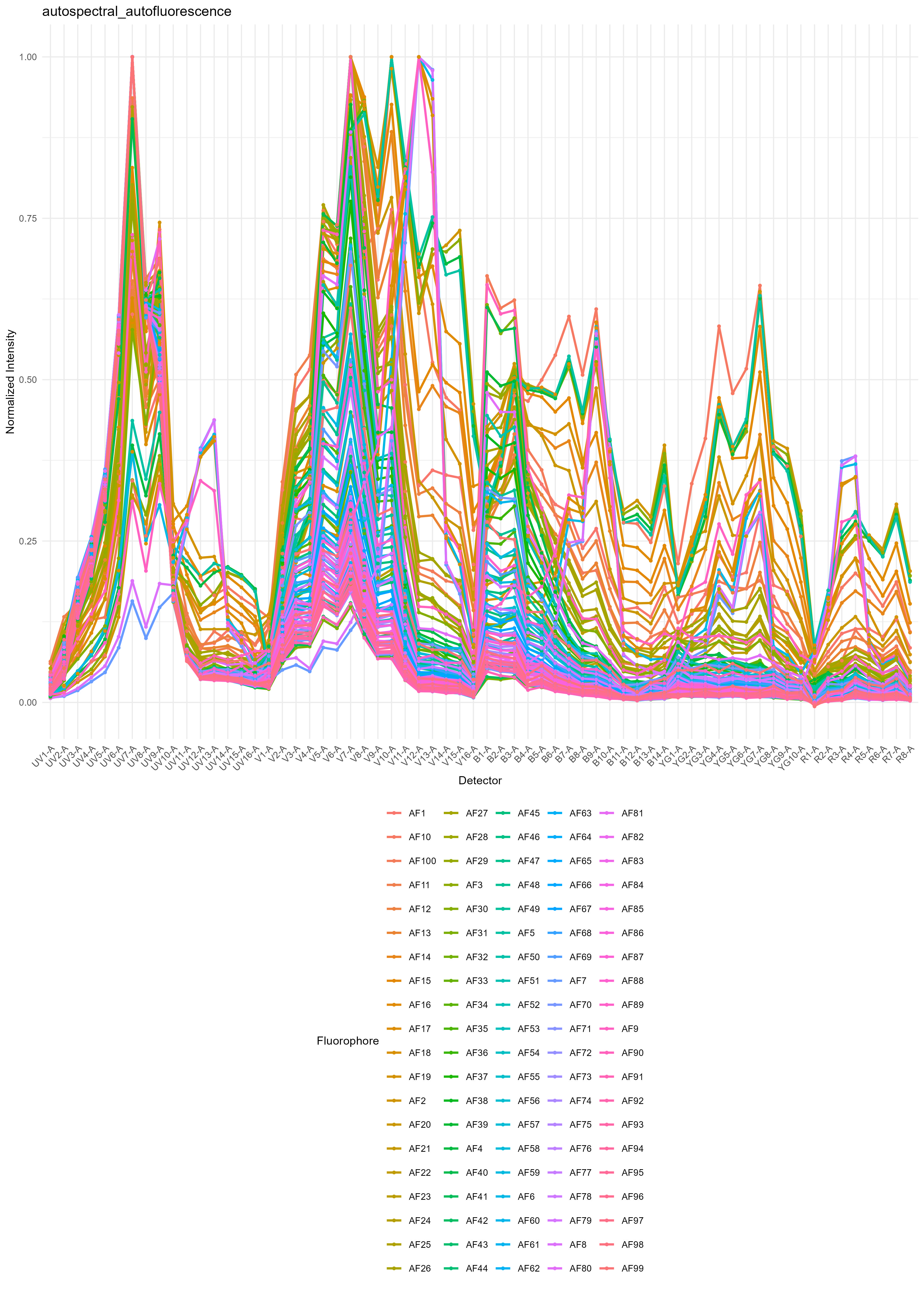
          file.suffix = "per-cell AF extraction")

We get the distribution of autofluorescence spectra as a spectral trace and as a heatmap in figure_autofluorescence. The AF spectra are saved as a CSV file in table_spectra.

Spleen AF

If you want to do this with samples containing different autofluorescence profiles, such as we have here, we extract the AF spectral variation from each type of unstained sample. We then provide the corresponding af.spectra to each unmixing call. The unmixing call can be to a single FCS file, or it can be, as above, to a folder. So, if you have a whole set of stained lung samples, you’d pull your AF spectra from the unstained lung sample, and then call unmix.folder on the folder containing your lung (and only lung) samples. Repeat for each type of autofluorescence sample.

In this case, we have three types of samples: spleen, liver and lung tissues. If you are working with human PBMCs, usually a single (optionally pooled) unstained PBMC sample is fine. If, however, you have samples from very sick donors, you might consider collecting unstained sample from each donor and matching the autofluorescence more closely.

lung.unstained <- "./Raw/Set1/Unstained/D2 Lung_Set1.fcs"
lung.af <- get.af.spectra(lung.unstained, asp, spectra)
lung.fcs.file <- "./Raw/Set1/Stained/D5 Lung_Set1.fcs"
unmix.fcs(lung.fcs.file, spectra, asp, flow.control,
          method = "AutoSpectral", af.spectra = lung.af,
          file.suffix = "per-cell AF extraction")

liver.unstained <- "./Raw/Set1/Unstained/D3 Liver_Set1.fcs"
liver.af <- get.af.spectra(liver.unstained, asp, spectra)
liver.fcs.file <- "./Raw/Set1/Stained/D6 Liver_Set1.fcs"
unmix.fcs(liver.fcs.file, spectra, asp, flow.control,
          method = "AutoSpectral", af.spectra = liver.af,
          file.suffix = "per-cell AF extraction")

To do per-cell fluorophore optimization, we will first measure the variation in the spectrum for each fluorophore. For the unmixing, we’ll supply the af.spectra and the spectra.variants, calling AutoSpectral unmixing. For best results, you should install AutoSpectralRcpp, for which you will need Rtools.

devtools::install_github("DrCytometer/AutoSpectralRcpp")

We provide spleen.af as the af.spectra here because the control samples are from spleen. Provide whatever is the best fit for your single-stained controls.

variants <- get.spectral.variants(control.dir, control.file, asp, spectra,
                                  af.spectra = spleen.af, parallel = TRUE)

The output of this is saved as an RDS file in folder figure_spectral_variants. You can load it back in using the readRDS() function in base R.

There are plots of the spectral variation for each fluorophore. For something like the CD11b-BUV805 in this data, the variation is largely changes in the autofluorescence because there are multiple cell types expressing CD11b.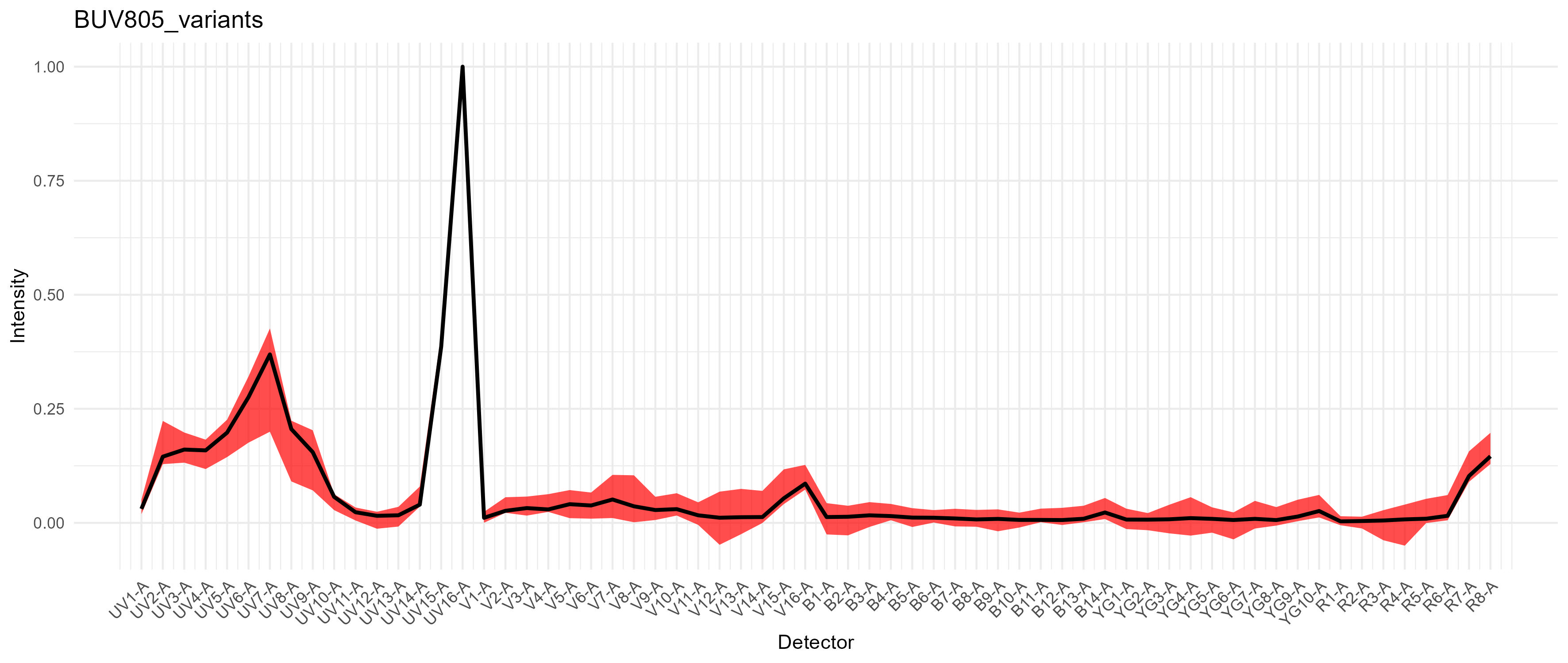

For PE-Cy7, we get a modest difference in the excitation between the blue and yellow-green lasers, which would cause spread if we had a fluorophore in that range on the blue laser, such as RB780. We don’t in this case.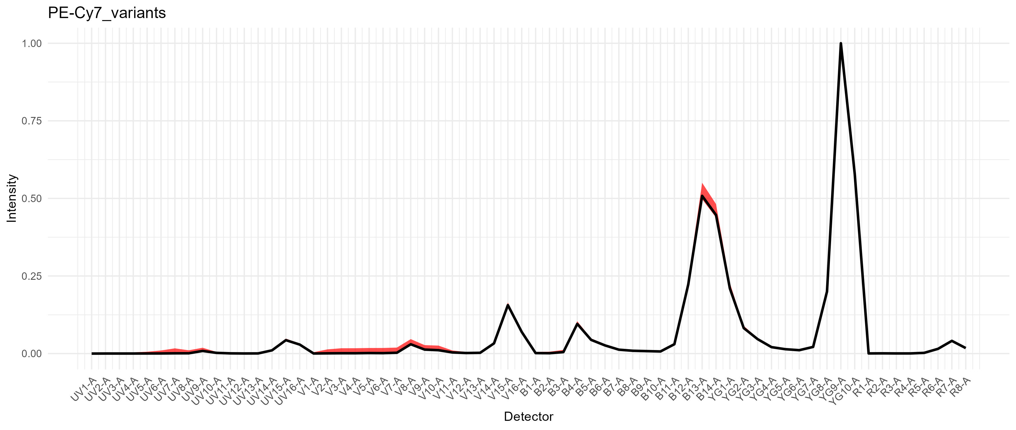

We can now pass this to the unmixing call. For best results, we’ll set the speed to slow, which recalculates the unmixing matrix for each variant. This can be a bit slow. Parallelization is automatic here if you have installed AutoSpectralRcpp. If you are using base R only, try turning on the parallel=TRUE.

unmix.fcs(lung.fcs.file, spectra, asp, flow.control,
          method = "AutoSpectral", af.spectra = lung.af,
          spectra.variants = variants,
          file.suffix = "per-cell AF and fluorophore optimization",
          speed = "slow")

Please note that if you are comparing the output FCS files from AutoSpectral to others you may have from the cytometer and you are doing this in FlowJo, FlowJo V10 is still terrible at handling scales. You must set the transformations on the axes to be the same for all coefficients in order to do a fair comparison. Otherwise you’ll see whatever you’ve already done to tune your display (e.g., biexponential width basis) for your existing files versus some random default selection by FlowJo for AutoSpectral’s files. Nothing to do with me.

You can do a comparison using the plotting functions in AutoSpectral, but a dedicated flow cytometry analysis program with a graphical interface will be better.

autospectral.unmixed.lung <- "AutoSpectral_unmixed/D5 Lung_Set1 AutoSpectral per-cell AF and fluorophore optimization.fcs"
spectroflo.unmixed.lung <- "./Unmixed/Set1/Stained/D5 Lung_Set1.fcs"

asp.lung <- flowCore::exprs(
  flowCore::read.FCS(autospectral.unmixed.lung,
                     truncate_max_range = FALSE)
  )
sf.lung <- flowCore::exprs(
  flowCore::read.FCS(spectroflo.unmixed.lung,
                     truncate_max_range = FALSE)
  )

create.biplot(sf.lung, "BUV395-A", "BV421-A", asp, title = "SpectroFlo")
create.biplot(asp.lung, "BUV395", "BV421", asp, title = "AutoSpectral")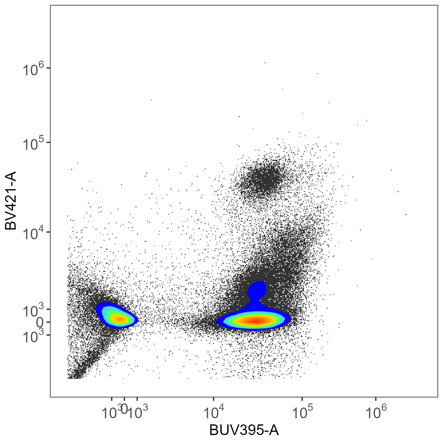

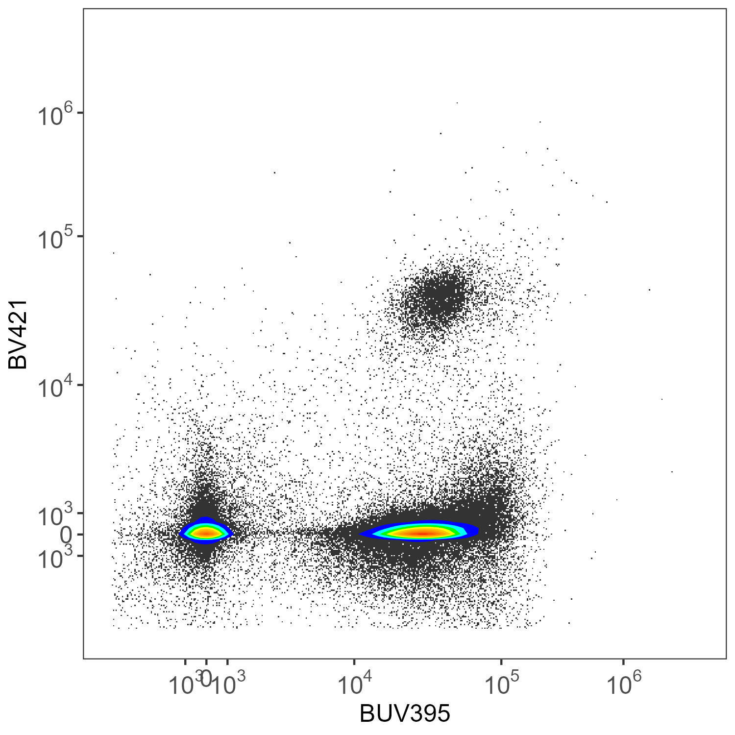
Here we have CD45-BUV395 and CD4-BV421. There really shouldn’t be much of anything low for CD4 in the mouse.