Creating the control file
Source:vignettes/articles/Control_File_example.Rmd
Control_File_example.RmdUpdate: there is now a Shiny app you can use to create your
control file. You may find this to be easier as it provides an
interactive interface much like a webpage. To use the app, download it
from AutoSpectral
App and place a copy of the app.r file in the folder
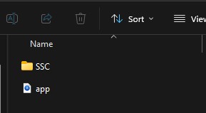
you’re working in. For easiest use, place the app file one level up from
the folder containing the single-stained control files, for example:
In this article, we’re going to cover how to create a control file, which is an essential first step in running AutoSpectral. The control file is a specifically formatted spreadsheet describing your single-stained control files. In the original AutoSpill, this needed to be created manually, but in AutoSpectral there is an option to fill in a lot of the information automatically. Let’s see how this works.
To start, we need to get the relevant parameters for the cytometer. This tells AutoSpectral a lot about what you’re doing. In this example, we’ll use data from the Cytek Aurora. These are the same data as in the Aurora_example article. https://data.mendeley.com/datasets/xzt3h3gnx9/1
asp <- get.autospectral.param(cytometer = "aurora")Create a folder containing only the single-stained control FCS files describe the path to that folder here.
control.dir <- "~/AutoSpectral_data/Aurora_example/Aurora_controls"With this information, we can create a draft of the control file.
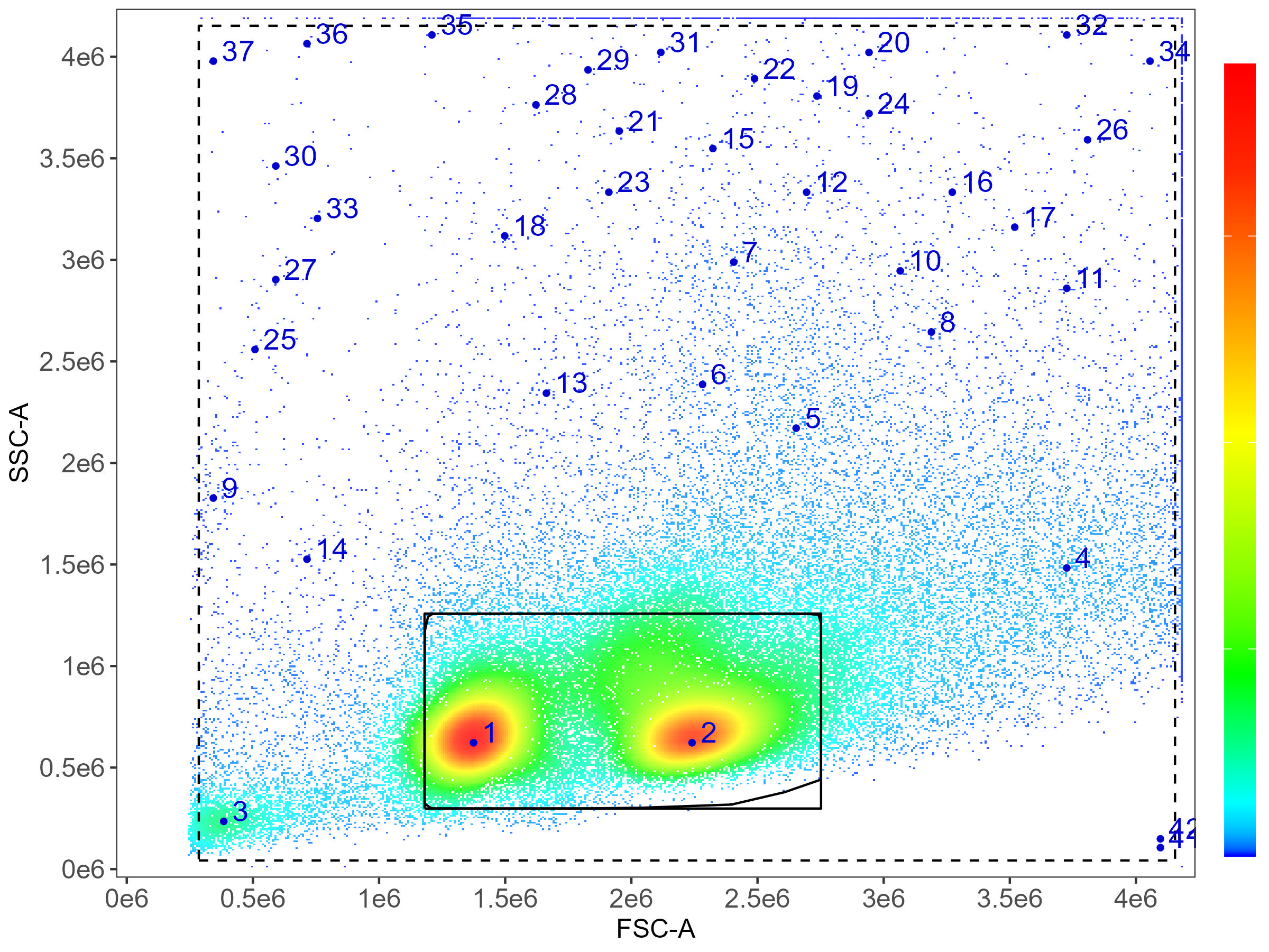
create.control.file(control.dir, asp)What this does is create a CSV file that in our case looks like this:
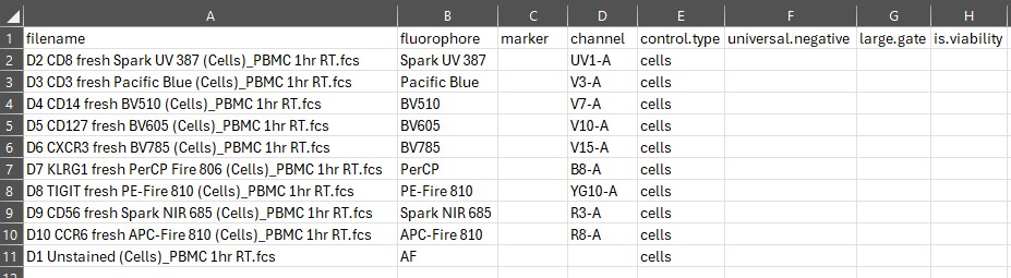
We get a list of all the fcs files in the folder
control.dir. These are in the filename column.
If you don’t see anything here, you’ve probably typed the path
incorrectly, but most likely in that case you’ll also get an error.
The next column is fluorophore. AutoSpectral has a
database (or in other words, a spreadsheet) of fluorophores and several
common synonyms for each. It’ll try to figure out the name of the
fluorophore in each of your single-stained controls and add this in the
corresponding fluorophore column. If you’re using a new
fluorophore that isn’t in the database, or you’ve called it something
odd like “Paficic blu3”, you’ll get No Match in the
fluorophore column. We’ll look at an example of this next. Any
No Match values must be changed–these are an indication
that you need to do the work yourself.
If you want, you can change the name of the fluorophore. Importantly,
the names in the fluorophore column is what will appear not
only any plots but also in the parameter names of the unmixed FCS
files.
After fluorophore, we have channel. This is
the “peak” channel for the fluorophore. If the fluorophore has been
found in the database, you should see something in the
channel column (and this should look appropriate for your
cytometer). If not, add the peak channel, which you can look up on
spectral viewer tools such as FluoroFinder, Cytek Cloud or BD Research
Cloud.
This channel does not actually need to be the peak channel for the
fluorophore, but it must be a channel that receives a good amount of
signal and provides separation from the negative population. Notice that
the Unstained sample does not get a channel assignment.
That’s fine. The Unstained cell sample will automatically
be used to generate a median autofluorescence signature, as you might
get with single-parameter autofluorescence extraction on most
cytometers. Don’t change the name of the Unstained cell
sample–leave it as AF.
Next, we have control.type. This is important to get
right. For Aurora samples, as part of a Reference Group, you
automatically get Cells or Beads as part of
the file name, and AutoSpectral will parse this, as it has done here.
For other platforms, you’ll need to enter the type of control for each
single-stained control. Beads and cells are treated a bit differently
for gating and autofluorecence handling, so you’ll get problems if you
put in the wrong type. Please stick to lower case, using either
cells or beads.
The final three columns will always need to be filled in manually.
For best results, you generally want to use a universal negative. In the
universal.negative column, copy and paste name of the
matching unstained sample from the filename column: 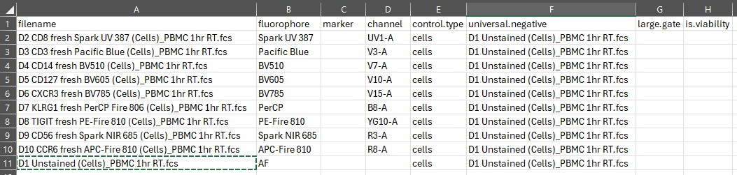
In this case, we only have one unstained sample because all the controls are from the same source: human PBMC.
The large.gate column provides a degree of control over
the automated gating. We’ll cover gating more extensively in another
article because that’s pretty complex, to be honest. What you need to
know here is whether your cells are small or big, basically. The default
gating is going to draw a rounded gate around the first dense population
to the right of the debris: 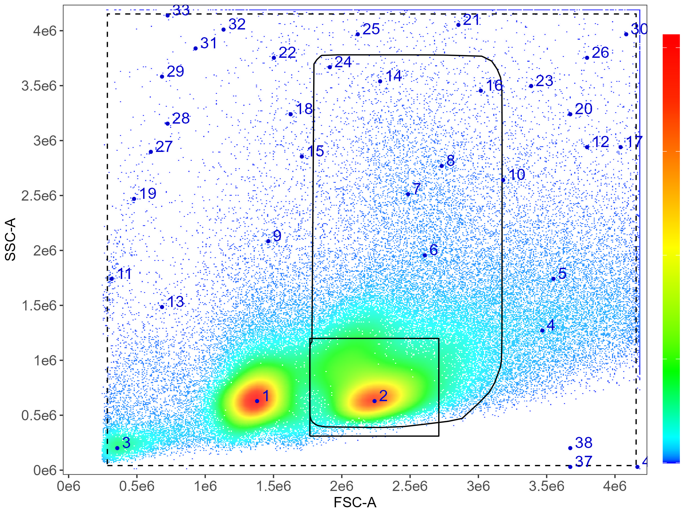
Here you can see that we’re mapping the density of events on FSC and
SSC. By default, the first population (1) is skipped, under the
assumption that this will normally be debris and/or dead cells. This can
be modified, see the gating article for details. Population 2 will be
the default target (square box), which works well in mouse and human
immunology where lymphocytes predominate. If your marker is expressed
primarily or at its highest level on cells that are bigger or more
granular, you need to set large.gate to TRUE.
This will then expand the gate as seen in the plot above with the curved
rectangular gate.
In the control file spreadsheet, we’re going to set
large.gate to TRUE for markers we know to be
on cells bigger than T cells. If you don’t know, you can open your
controls in a tool such as FlowJo or FCSExpress and plot the peak
channel for your marker versus SSC (or check on some unmixed data).
Setting Large Gate options: 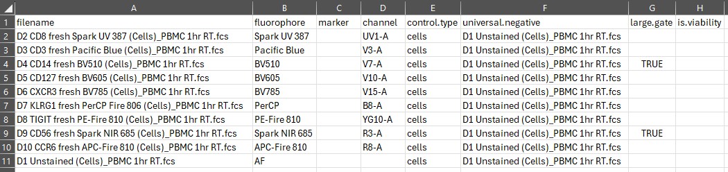
Note that CD56 cells, particularly the CD56-bright cells, tend to be a bit higher on SSC than the T lymphocytes.
CD8 T cell gating: 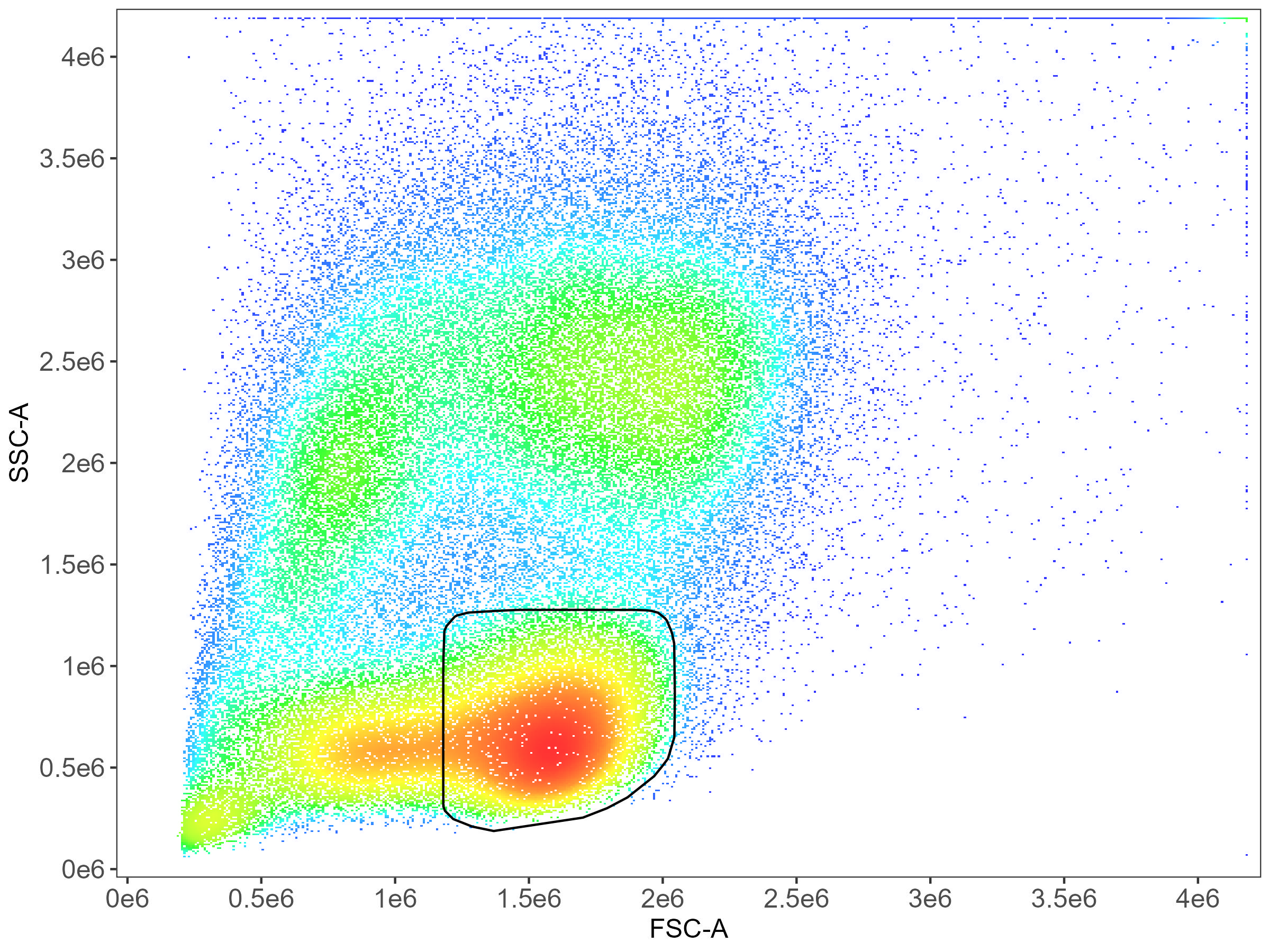
CD14 monocyte gating: 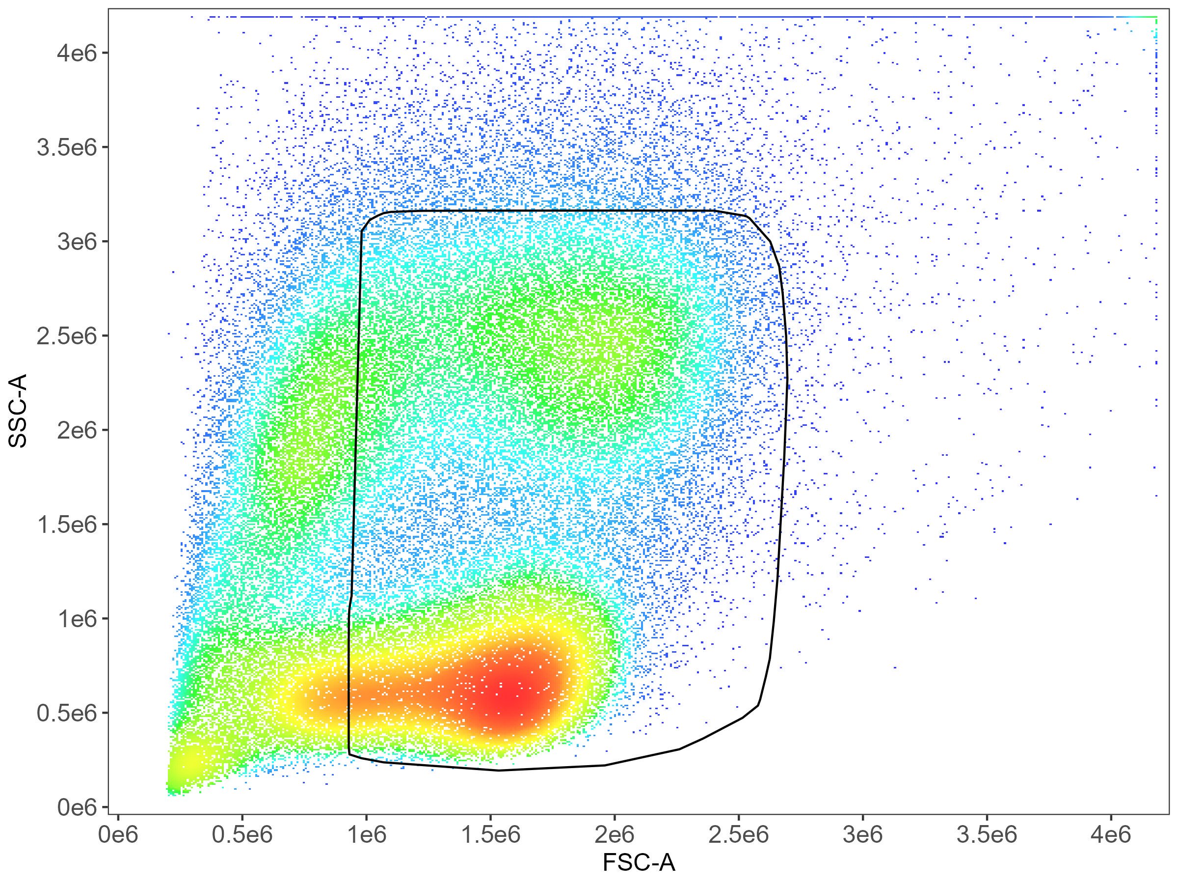
Finally, we get to the is.viability column. This dataset
doesn’t have a viability dye (ooh, not good!). This means we don’t put
anything in this column. If we had a viability dye, we would put
TRUE in the is.viability column for that
control. This affects the gating, extending the gate to the left on FSC
to include more dead cells, as we can see in this example of mostly dead
mouse splenocytes:
Whatever you’ve named your control file (the default output is
fcs_control_file.csv), you’ll need to tell AutoSpectral
what it’s called:
control.file <- "fcs_control_file.csv"To confirm that everything is set up correctly, and to check for a
multitude of other potential problems, AutoSpectral contains this handy
helper function called check.control.file. This actually
checks your single-stained control FCS files as well to be sure that
they’re all consistent with each other. This outputs the list of
critical errors (things that will probably stop AutoSpectral from
running) and warnings (things to check–did you mean to set it up that
way?) as a message to the screen and also returns it as an object. So,
if there are a lot of errors, you can review the list again. Note that
check.control.file runs inside of
define.flow.control with a strict setting that will cause
it to abort if it finds anything it deems to be an error. So, fix the
errors first.
potential.problems <- check.control.file(control.dir, control.file, asp)For this dataset, the control file is now complete and we are ready to run AutoSpectral.
If you happen to run create.control.file again, it will
create another blank control file spreadsheet with an incrementing file
number. This ensures that it doesn’t overwrite your existing filled-in
control file.
Haven’t done this yet, sorry In the next article, we’ll look at how to create a control file for a more complex experiment where we have beads and cells, different universal negatives and, ideally, a viability marker. We’ll also see what to do when your fluorophores can’t be found in the database.